Posted by Stephan Rasp, Research Scientist, and Carla Bromberg, Program Lead, Google Research
In 1950, weather forecasting started its digital revolution when researchers used the first programmable, general-purpose computer ENIAC to solve mathematical equations describing how weather evolves. In the more than 70 years since, continuous advancements in computing power and improvements to the model formulations have led to steady gains in weather forecast skill: a 7-day forecast today is about as accurate as a 5-day forecast in 2000 and a 3-day forecast in 1980. While improving forecast accuracy at the pace of approximately one day per decade may not seem like a big deal, every day improved is important in far reaching use cases, such as for logistics planning, disaster management, agriculture and energy production. This “quiet” revolution has been tremendously valuable to society, saving lives and providing economic value across many sectors.
Now we are seeing the start of yet another revolution in weather forecasting, this time fueled by advances in machine learning (ML). Rather than hard-coding approximations of the physical equations, the idea is to have algorithms learn how weather evolves from looking at large volumes of past weather data. Early attempts at doing so go back to 2018 but the pace picked up considerably in the last two years when several large ML models demonstrated weather forecasting skill comparable to the best physics-based models. Google’s MetNet [1, 2], for instance, demonstrated state-of-the-art capabilities for forecasting regional weather one day ahead. For global prediction, Google DeepMind created GraphCast, a graph neural network to make 10 day predictions at a horizontal resolution of 25 km, competitive with the best physics-based models in many skill metrics.
Apart from potentially providing more accurate forecasts, one key advantage of such ML methods is that, once trained, they can create forecasts in a matter of minutes on inexpensive hardware. In contrast, traditional weather forecasts require large super-computers that run for hours every day. Clearly, ML represents a tremendous opportunity for the weather forecasting community. This has also been recognized by leading weather forecasting centers, such as the European Centre for Medium-Range Weather Forecasts’ (ECMWF) machine learning roadmap or the National Oceanic and Atmospheric Administration’s (NOAA) artificial intelligence strategy.
To ensure that ML models are trusted and optimized for the right goal, forecast evaluation is crucial. Evaluating weather forecasts isn’t straightforward, however, because weather is an incredibly multi-faceted problem. Different end-users are interested in different properties of forecasts, for example, renewable energy producers care about wind speeds and solar radiation, while crisis response teams are concerned about the track of a potential cyclone or an impending heat wave. In other words, there is no single metric to determine what a “good” weather forecast is, and the evaluation has to reflect the multi-faceted nature of weather and its downstream applications. Furthermore, differences in the exact evaluation setup — e.g., which resolution and ground truth data is used — can make it difficult to compare models. Having a way to compare novel and established methods in a fair and reproducible manner is crucial to measure progress in the field.
To this end, we are announcing WeatherBench 2 (WB2), a benchmark for the next generation of data-driven, global weather models. WB2 is an update to the original benchmark published in 2020, which was based on initial, lower-resolution ML models. The goal of WB2 is to accelerate the progress of data-driven weather models by providing a trusted, reproducible framework for evaluating and comparing different methodologies. The official website contains scores from several state-of-the-art models (at the time of writing, these are Keisler (2022), an early graph neural network, Google DeepMind’s GraphCast and Huawei’s Pangu-Weather, a transformer-based ML model). In addition, forecasts from ECMWF’s high-resolution and ensemble forecasting systems are included, which represent some of the best traditional weather forecasting models.
Making evaluation easier
The key component of WB2 is an open-source evaluation framework that allows users to evaluate their forecasts in the same manner as other baselines. Weather forecast data at high-resolutions can be quite large, making even evaluation a computational challenge. For this reason, we built our evaluation code on Apache Beam, which allows users to split computations into smaller chunks and evaluate them in a distributed fashion, for example using DataFlow on Google Cloud. The code comes with a quick-start guide to help people get up to speed.
Additionally, we provide most of the ground-truth and baseline data on Google Cloud Storage in cloud-optimized Zarr format at different resolutions, for example, a comprehensive copy of the ERA5 dataset used to train most ML models. This is part of a larger Google effort to provide analysis-ready, cloud-optimized weather and climate datasets to the research community and beyond. Since downloading these data from the respective archives and converting them can be time-consuming and compute-intensive, we hope that this should considerably lower the entry barrier for the community.
Assessing forecast skill
Together with our collaborators from ECMWF, we defined a set of headline scores that best capture the quality of global weather forecasts. As the figure below shows, several of the ML-based forecasts have lower errors than the state-of-the-art physical models on deterministic metrics. This holds for a range of variables and regions, and underlines the competitiveness and promise of ML-based approaches.
This scorecard shows the skill of different models compared to ECMWF’s Integrated Forecasting System (IFS), one of the best physics-based weather forecasts, for several variables. IFS forecasts are evaluated against IFS analysis. All other models are evaluated against ERA5. The order of ML models reflects publication date.
Toward reliable probabilistic forecasts
However, a single forecast often isn’t enough. Weather is inherently chaotic because of the butterfly effect. For this reason, operational weather centers now run ~50 slightly perturbed realizations of their model, called an ensemble, to estimate the forecast probability distribution across various scenarios. This is important, for example, if one wants to know the likelihood of extreme weather.
Creating reliable probabilistic forecasts will be one of the next key challenges for global ML models. Regional ML models, such as Google’s MetNet already estimate probabilities. To anticipate this next generation of global models, WB2 already provides probabilistic metrics and baselines, among them ECMWF’s IFS ensemble, to accelerate research in this direction.
As mentioned above, weather forecasting has many aspects, and while the headline metrics try to capture the most important aspects of forecast skill, they are by no means sufficient. One example is forecast realism. Currently, many ML forecast models tend to “hedge their bets” in the face of the intrinsic uncertainty of the atmosphere. In other words, they tend to predict smoothed out fields that give lower average error but do not represent a realistic, physically consistent state of the atmosphere. An example of this can be seen in the animation below. The two data-driven models, Pangu-Weather and GraphCast (bottom), predict the large-scale evolution of the atmosphere remarkably well. However, they also have less small-scale structure compared to the ground truth or the physical forecasting model IFS HRES (top). In WB2 we include a range of these case studies and also a spectral metric that quantifies such blurring.
Forecasts of a front passing through the continental United States initialized on January 3, 2020. Maps show temperature at a pressure level of 850 hPa (roughly equivalent to an altitude of 1.5km) and geopotential at a pressure level of 500 hPa (roughly 5.5 km) in contours. ERA5 is the corresponding ground-truth analysis, IFS HRES is ECMWF’s physics-based forecasting model.
Conclusion
WeatherBench 2 will continue to evolve alongside ML model development. The official website will be updated with the latest state-of-the-art models. (To submit a model, please follow these instructions). We also invite the community to provide feedback and suggestions for improvements through issues and pull requests on the WB2 GitHub page.
Designing evaluation well and targeting the right metrics is crucial in order to make sure ML weather models benefit society as quickly as possible. WeatherBench 2 as it is now is just the starting point. We plan to extend it in the future to address key issues for the future of ML-based weather forecasting. Specifically, we would like to add station observations and better precipitation datasets. Furthermore, we will explore the inclusion of nowcasting and subseasonal-to-seasonal predictions to the benchmark.
We hope that WeatherBench 2 can aid researchers and end-users as weather forecasting continues to evolve.
Acknowledgements
WeatherBench 2 is the result of collaboration across many different teams at Google and external collaborators at ECMWF. From ECMWF, we would like to thank Matthew Chantry, Zied Ben Bouallegue and Peter Dueben. From Google, we would like to thank the core contributors to the project: Stephan Rasp, Stephan Hoyer, Peter Battaglia, Alex Merose, Ian Langmore, Tyler Russell, Alvaro Sanchez, Antonio Lobato, Laurence Chiu, Rob Carver, Vivian Yang, Shreya Agrawal, Thomas Turnbull, Jason Hickey, Carla Bromberg, Jared Sisk, Luke Barrington, Aaron Bell, and Fei Sha. We also would like to thank Kunal Shah, Rahul Mahrsee, Aniket Rawat, and Satish Kumar. Thanks to John Anderson for sponsoring WeatherBench 2. Furthermore, we would like to thank Kaifeng Bi from the Pangu-Weather team and Ryan Keisler for their help in adding their models to WeatherBench 2.
NVIDIA Jetson Orin is the best-in-class embedded platform for AI workloads. One of the key components of the Orin platform is the second-generation Deep…
NVIDIA Jetson Orin is the best-in-class embedded platform for AI workloads. One of the key components of the Orin platform is the second-generation Deep Learning Accelerator (DLA), the dedicated deep learning inference engine that offers one-third of the AI compute on the AGX Orin platforms.
This post is a deep technical dive into how embedded developers working with Orin platforms can deploy deep neural networks (DNNs) using YOLOv5 as a reference. To learn more about how DLA can help maximize the performance of your deep learning applications, see Maximizing Deep Learning Performance on NVIDIA Jetson Orin with DLA.
YOLOv5 is an object detection algorithm. Building on the success of v3 and v4, YOLOv5 aims to provide improved accuracy and speed in real-time object detection tasks. YOLOv5 has gained notoriety due to its excellent trade-off between accuracy and speed, making it a popular choice among researchers and practitioners in the field of computer vision. Its open-source implementation enables developers to leverage pretrained models and customize them according to specific goals.
Train a YOLOv5 model with Quantization-Aware Training (QAT) and export it for deployment on DLA.
Deploy the network and run inference using CUDA through TensorRT and cuDLA.
Execute on-target YOLOv5 accuracy validation and performance profiling.
Using this sample, we demonstrate how to achieve 37.3 mAP on the COCO dataset with DLA INT8 (official FP32 mAP is 37.4). We also show how to obtain over 400 FPS for YOLOv5 on a single NVIDIA Jetson Orin DLA. (A total of two DLA instances are available on Orin.)
QAT training and export for DLA
To balance the inference performance and accuracy of YOLOv5, it’s essential to apply Quantization-Aware-Training (QAT) on the model. Because DLA does not support QAT through TensorRT at the time of writing, it’s necessary to convert the QAT model to a Post-Training Quantization (PTQ) model before inference. The steps are outlined in Figure 1.
Figure 1. Key steps involved in converting a QAT model to a PTQ model
QAT training workflow
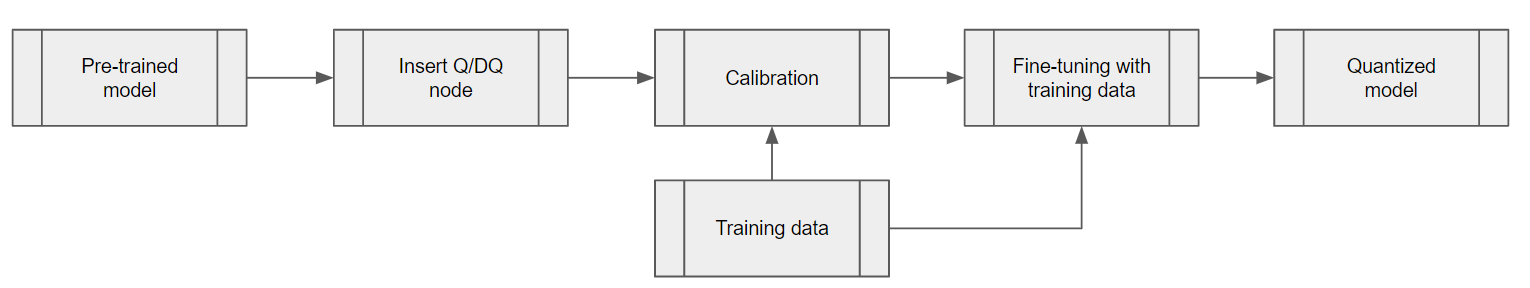
Use the TensorRT pytorch-quantization toolkit to quantize YOLOv5. The first step is to add quantizer modules to the neural network graph. This toolkit provides a set of quantized layer modules for common DL operations. If a module is not among the provided quantized modules, you can create a custom quantization module for the right place in the model.
The second step is to calibrate the model, obtaining the scale values for each Quantization/Dequantization (Q/DQ) module. After the calibration is complete, select a training schedule and fine-tune the calibrated model using the COCO dataset.
Figure 2. Steps of the QAT training workflow
Adding Q/DQ nodes
There are two options for adding Q/DQ nodes to your network:
Option 1: Place Q/DQ nodes, as recommended, in TensorRT Processing of Q/DQ Networks. This method follows TensorRT fusion strategy for Q/DQ layers. These TensorRT strategies are mostly tuned for GPU inference. To make this compatible with DLA, add additional Q/DQ nodes, which can be derived using the scales from their neighboring layers with the Q/DQ Translator.
Any missing scales would otherwise result in certain layers running in FP16. This may result in a slight decrease in mAP and possibly a large performance drop. The Orin DLA is optimized for INT8 convolutions, about 15x over FP16 dense performance (or 30x when comparing dense FP16 to INT8 sparse performance).
Option 2: Insert Q/DQ nodes at every layer to make sure all tensors have INT8 scales. With this option, all layers’ scales can be obtained during model fine-tuning. However, this method may potentially disrupt TensorRT fusion strategy with Q/DQ layers when running inference on GPU and lead to higher latency on the GPU. For DLA, on the other hand, the rule of thumb with PTQ scales is, “The more available scales, the lower the latency.”
As confirmed by experiment, our YOLOv5 model was verified on the COCO 2017 validation dataset with a resolution of 672 x 672 pixels. Option 1 and Option 2, respectively, achieved mAP scores of 37.1 and 37.0.
Choose the best option based on your needs. If you already have an existing QAT workflow for GPU and would like to preserve it as much as possible, Option 1 is probably better. (You may need to extend Q/DQ Translator to infer more missing scales to achieve optimal DLA latency as well.)
On the other hand, if you are looking for a QAT training method that inserts Q/DQ nodes into all layers and is compatible with DLA, Option 2 may be your most promising.
Q/DQ Translator workflow
The purpose of the Q/DQ Translator is to translate an ONNX graph trained with QAT, to PTQ tensor scales and an ONNX model without Q/DQ nodes.
For this YOLOv5 model, extract quantization scales from Q/DQ nodes in the QAT model. Use the information of neighboring layers to infer the input/output scales of other layers such as Sigmoid and Mul in YOLOv5’s SiLU or for Concat nodes. After scales are extracted, export the ONNX model without Q/DQ nodes and the (PTQ) calibration cache file such that TensorRT can use them to build a DLA engine.
Deploying network to DLA for inference
The next step is to deploy the network and run inference using CUDA through TensorRT and cuDLA.
Loadable build with TensorRT
Use TensorRT to build the DLA loadable. This provides an easy-to-use interface for DLA loadable building and seamless integration with GPU if needed. For more information about TensorRT-DLA, see Working with DLA in the TensorRT Developer Guide.
trtexec is a convenient tool provided by TensorRT for building engines and benchmarking performance. Note that a DLA loadable is the result of successful DLA compilation through the DLA Compiler, and that TensorRT can package DLA loadables inside of serialized engines.
First, prepare the ONNX model and the calibration cache generated in the previous section. The DLA loadable can be built with a single command. Pass the --safe option and the entire model can run on DLA. This directly saves the compilation result as a serialized DLA loadable (without a TensorRT engine wrapping around it). For more details about this step, see the NVIDIA Deep Learning TensorRT Documentation.
Note that the input format dla_hwc4 is highly recommended from a performance point of view, if your model input qualifies. The input must have at most four input channels and be consumed by a convolution. In INT8, DLA can benefit from a specific hardware and software optimization that is not available if you use --inputIOFormats=int8:chw32 instead, for example.
Running inference using cuDLA
cuDLA is the CUDA runtime interface for DLA, an extension of the CUDA programming model that integrates DLA with CUDA. cuDLA enables you to submit DLA tasks using CUDA programming constructs. You can run inference using cuDLA either implicitly through TensorRT runtime or you can explicitly call the cuDLA APIs. This sample demonstrates the latter approach to explicitly call cuDLA APIs to run inference in hybrid mode and standalone mode.
cuDLA hybrid mode and standalone mode mainly differ in synchronization. In hybrid mode, DLA tasks are submitted to a CUDA stream, so synchronization can be done seamlessly with other CUDA tasks.
In standalone mode, the cudlaTask structure has a provision to specify wait and signal events that cuDLA must wait on and signal respectively, as part of cudlaSubmitTask.
In short, using cuDLA hybrid mode can give quick integration with other CUDA tasks. Using cuDLA standalone mode can prevent the creation of CUDA context, and thus can save resources if the pipeline has no CUDA context.
The primary cuDLA APIs used in this YOLOv5 sample are detailed below.
cudaMalloc and cudlaMemRegister are called to first allocate memory on GPU, then let the CUDA pointer be registered with the DLA. (Used only for hybrid mode.)
cudlaSubmitTask is called to submit the inference task. In hybrid mode, users need to specify the CUDA stream to let cuDLA tasks run on it. In standalone mode, users need to specify the signal event and wait event to let cuDLA wait and signal when the corresponding fence expires.
On-target validation and profiling
It’s important to note the numerical differences between GPU to DLA. The underlying hardware is different, so the computations are not bit-wise accurate. Because training the network is done on the GPU and then deployed to DLA on the target, it’s important to validate on the target. This specifically comes into play when it comes to quantization. It’s also important to compare against a reference baseline.
YOLOv5 DLA accuracy validation
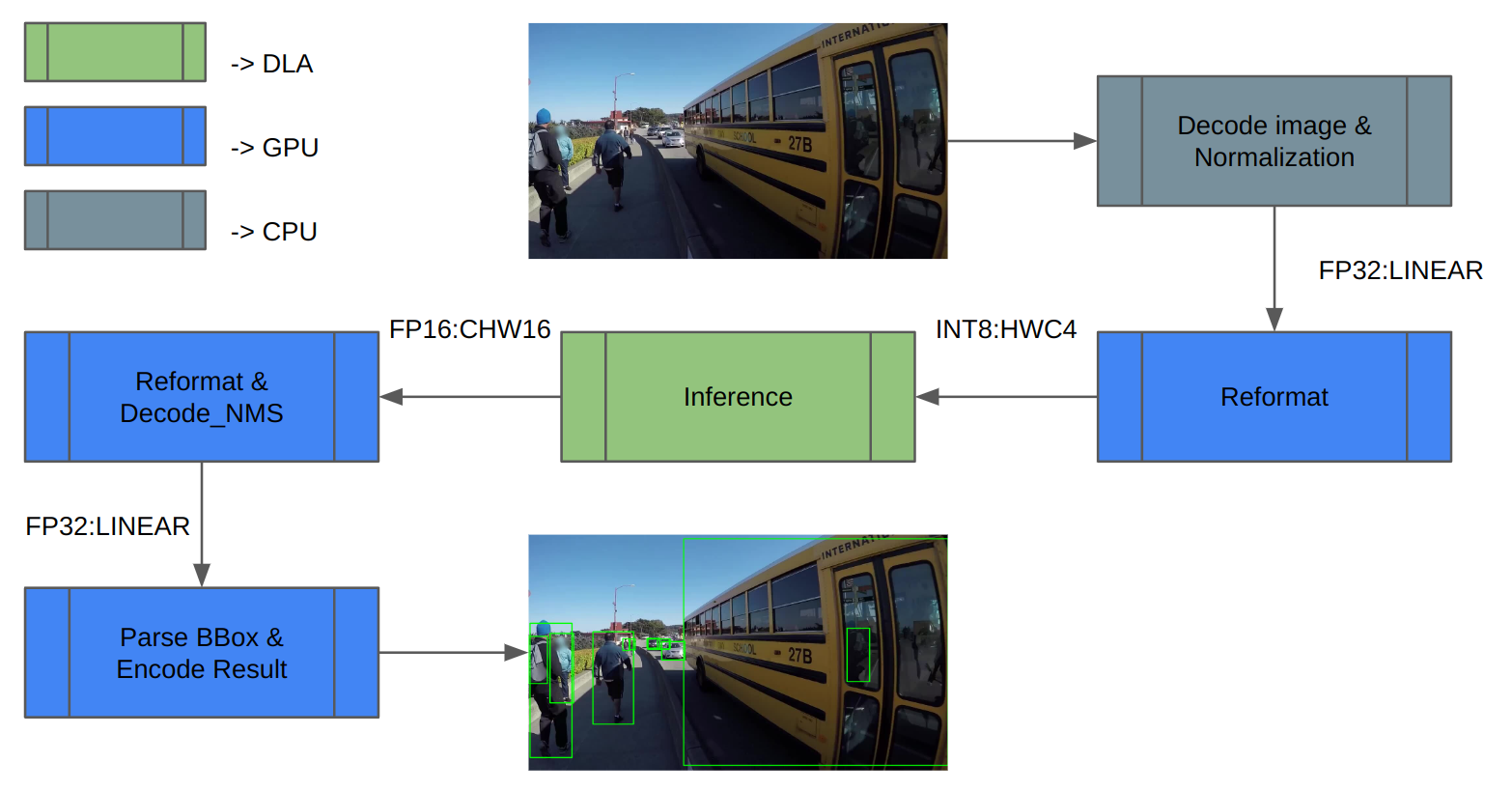
We used the COCO dataset to validate. Figure 3 shows the inference pipeline architecture. First, load the image data and normalize it. Extra reformats on the inference inputs and outputs are needed because DLA only supports INT8/FP16.
After inference, decode the inference result and perform NMS (non-maximum suppression) to get the detection result. Finally, save the result and compute mAP.
Figure 3. Inference pipeline with tasks mapped to the different compute engines
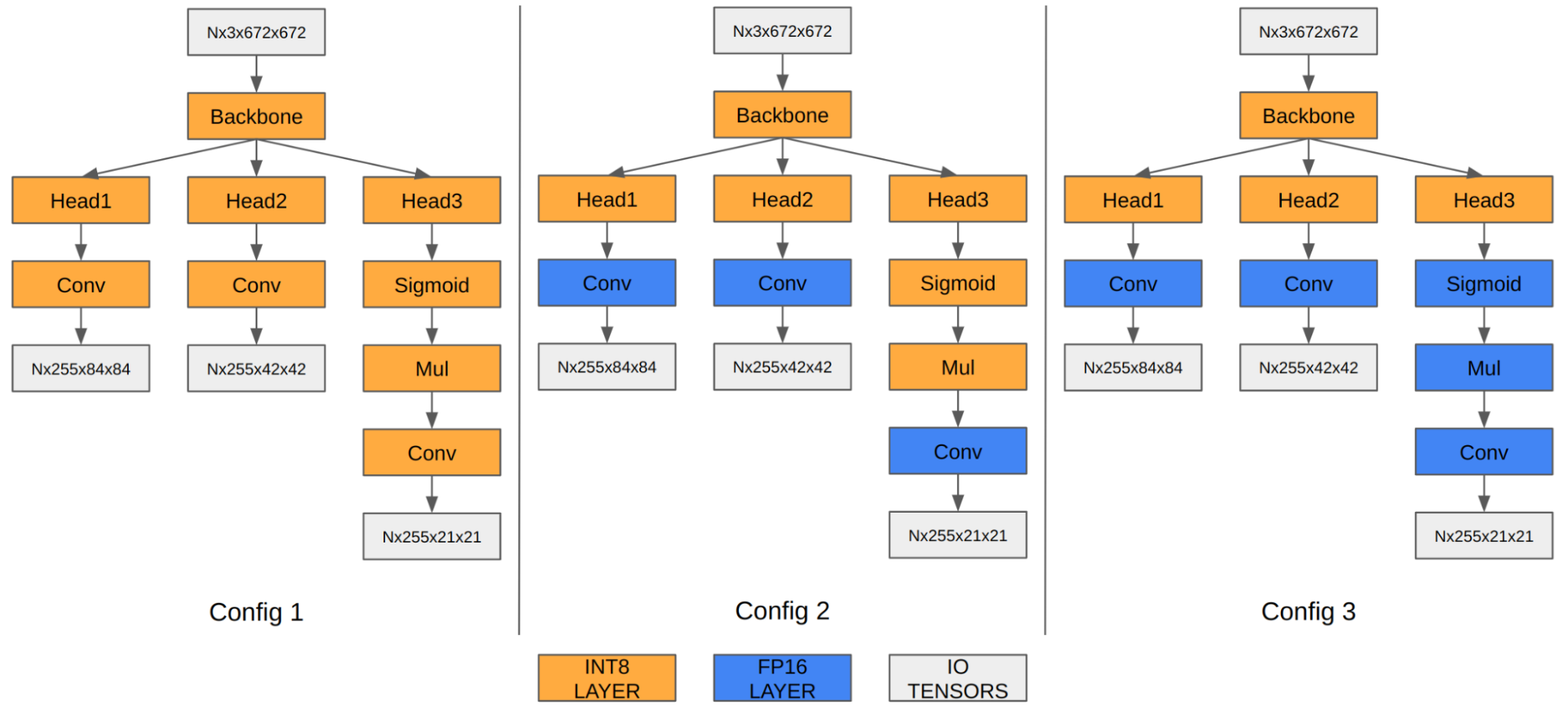
In the case of YOLOv5, the feature maps of the last three convolution layers encode final detection information. When quantized to INT8, the quantization error of the bounding box coordinates becomes noticeable compared to FP16/FP32, thus affecting the final mAP.
Our experiment shows that running the last three convolution layers in FP16 improves the final mAP from 35.9 to 37.1. Orin DLA has a special hardware design highly optimized for INT8, so we observe a performance drop when these three convolutions run in FP16.
Figure 4. YOLOv5 engine with different precision configurations
Table 1. Configurations exploring mixed precision for the last three convolution layers
Note that the mAP results are based on Option 1 described in the preceding section on adding Q/DQ nodes. You can apply the same principle to Option 2 as well.
YOLOv5 DLA performance
DLA offers one-third of AI compute on Orin AGX platforms, thanks to the two DLA cores. For a general baseline of Orin DLA performance, see Deep-Learning-Accelerator-SW on GitHub.
In the latest release, DLA 3.14.0 (DOS 6.0.8.0 and JetPack 6.0), several performance optimizations were added to the DLA compiler that specifically apply for INT8 CNN architecture-based models:
Native INT8 Sigmoid (previously ran in FP16 and had to be cast to and from INT8; also applies to Tanh)
INT8 SiLU fusion into a single DLA HW operation (instead of standalone Sigmoid plus standalone elementwise Mul)
Fusing the INT8 SiLU HW op with the previous INT8 Conv HW op (also applies to standalone Sigmoid or Tanh)
These improvements can provide a 6x speedup for YOLO architectures compared to prior releases. For instance, in the case of YOLOv5, the inference performance jumped from 13 ms to 2.4 ms in INT8 (with a few layers running in FP16), which is a 5.4x improvement. Further, you can use the cuDLA sample to profile your DNN layer-wise, identify bottlenecks, and modify your network to improve its performance.
Get started with DLA
This post explains how to run an entire object detection pipeline on Orin in the most efficient way using YOLOv5 on its dedicated Deep Learning Accelerator. Keep in mind that other SoC components such as the GPU are either idling or running at very small load. If you had a single camera producing inputs at 30 fps, one DLA instance would only be loaded at about 10%. So there is plenty of headroom for adding more bells and whistles to your application.
Ready to dive in? The YOLOv5 sample replicates the entire workflow discussed here. You can use it as a reference point for your own use case.
For beginners, the Jetson_dla_tutorial on GitHub demonstrates a basic DLA workflow to help you get started deploying a simple model to DLA.
Ray and path tracing algorithms construct light paths by starting at the camera or the light sources and intersecting rays with the scene geometry. As objects…
Ray and path tracing algorithms construct light paths by starting at the camera or the light sources and intersecting rays with the scene geometry. As objects are hit, new secondary rays are generated on these surfaces to continue the paths.
In theory, these secondary rays will not yield an intersection with the same triangle again, as intersections at a distance of zero are excluded by the intersection algorithm. In practice, however, the finite floating-point precision used in the actual implementation often leads to false-positive results, known as self-intersections (Figure 2). This creates artifacts, such as shadow acne, where the triangle sometimes improperly shadows itself (Figure 1).
Self-intersection can be avoided by explicitly excluding the same primitive from intersection using its identifier. In DirectX Raytracing (DXR) this self-intersection check would be implemented in an any-hit shader. However, forcing an any-hitinvocation for all triangle hits comes at a significant performance penalty. Furthermore, this method does not deal with false positives against adjacent (near) coplanar triangles.
The most widespread solutions to work around the issue use various heuristics to offset the ray along either the ray direction or the normal. These methods are, however, not robust enough to handle a variety of common production content and may even require manual parameter tweaking on a per-scene basis, particularly in scenes with heavily translated, scaled or sheared instanced geometry. For more information, see Ray Tracing Gems: High-Quality and Real-Time Rendering with DXR and Other APIs.
Alternatively, the sources of the numerical imprecision can be numerically bounded at runtime, giving robust error intervals on the intersection test. However, this comes with considerable performance overhead and requires source access to the underlying implementation of the ray/triangle intersection routine, which is not possible in a hardware-accelerated API like DXR.
This post describes a robust offsetting method for secondary rays spawned from triangles in DXR. The method is based on a thorough numerical analysis of the sources of the numerical imprecision. It involves computing spawn points for secondary rays, safe from self-intersections. The method does not require modification of the traversal and ray/triangle intersection routines and can thus be used with closed-source and hardware-accelerated ray tracing APIs like DXR. Finally, the method does not rely on self-intersection rejection using an any-hit shader and has a fixed overhead per shading point.
Figure 1. Rendering with self-intersection avoidance (left) and without self-intersection avoidance (right). Image credit: Sander van der Meiren
Method overview
The spawn point of a secondary ray coincides with the hit point on a triangle of an incoming ray. The goal is to compute a spawn point as close as possible to the hit point in the triangle plane, while still avoiding self-intersections. Too close to the triangle may result in self-intersection artifacts, but too far away may push the spawn point past nearby geometry, causing light leaking artifacts.
Figure 2 shows the sources of numerical error for secondary rays. In the user shader, the object-space hit point is reconstructed and transformed into world-space. During DXR ray traversal, the world-space ray is transformed back into object-space and intersected against triangles.
Each of these operations accumulates numerical errors, possibly resulting in self-intersections. This method computes a minimal uncertainty interval centered around the intended ray origin (red dot in Figure 2) on the triangle at each operation. The approximate ray origin (black dot in Figure 2) lies within this uncertainty interval. The ray origin is offset along the triangle normal beyond the final uncertainty interval to prevent self-intersections.
Figure 2. The sources of numerical error in the user shader (left) and DXR ray traversal and intersection (right)
Hit point
Start by reconstructing the hit point and the geometric triangle normal in object-space (Listing 1).
precise float3 edge1 = v1 - v0;
precise float3 edge2 = v2 - v0;

// interpolate triangle using barycentrics
// add in base vertex last to reduce object-space error
precise float3 objPosition = v0 + mad(barys.x, edge1, mul(barys.y, edge2));
float3 objNormal = cross(edge1, edge2);
The hit point is computed by interpolating the triangle vertices v0, v1, and v2 using the 2D barycentric hit coordinates barys. Although it is possible to compute the interpolated hit point using two fused multiply-add operations, adding the base vertex v0 last reduces the maximum rounding error on the base vertex, which in practice dominates the rounding error in this computation.
Use the precise keyword to force the compiler to perform the computations exactly as specified. Enforced precise computation of the normal and the error bounds is not required. The effects of rounding errors on these quantities are vanishingly small and can safely be ignored for self-intersection.
Next, the object-space position is transformed into world-space (Listing 2).
Instead of using the HLSL matrix mul intrinsic, write out the transformation. This ensures that the translational part of the transformation is added last. This again reduces the rounding error on the translation, which in practice tends to dominate the error in this computation.
Finally, transform the object-space normal to world-space and normalize it (Listing 3).
const float3x4 w2o = WorldToObject3x4();

// transform normal to world-space using
// inverse transpose matrix
float3 wldNormal = mul(transpose((float3x3)w2o), objNormal);

// normalize world-space normal
const float wldScale = rsqrt(dot(wldNormal, wldNormal));
wldNormal = mul(wldScale, wldNormal);

// flip towards incoming ray
if(dot(WorldRayDirection(), wldNormal) > 0)
wldNormal = -wldNormal;
To support transformations with uneven scaling or shear, the normals are transformed using the inverse transpose transformation. There is no need to normalize the object-space normal before the transformation. It is necessary to normalize again in world-space anyway. Because the inverse length of the world normal is needed again later to appropriately scale the error bounds, normalize manually instead of using the HLSL normalize intrinsic.
Error bounds
With an approximate world-space position and triangle normal, continue by computing error bounds on the computed position, bounding the maximum finite precision rounding error. It is necessary to account for the rounding errors in the computations in Listings 1 and 2.
It is also necessary to account for rounding errors that may occur during traversal (Figure 2). During traversal, DXR will apply a world-to-object transformation and perform a ray-triangle intersection test. Both of these are performed in finite precision and thus introduce rounding errors.
Start by computing a combined object-space error bound, accounting both for the rounding errors in Listing 1 and rounding errors due to the DXR ray-triangle intersection test (Listing 4).
const float c0 = 5.9604644775390625E-8f;
const float c1 = 1.788139769587360206060111522674560546875E-7f;

// compute twice the maximum extent of the triangle
const float3 extent3 = abs(edge1) + abs(edge2) +
   abs(abs(edge1) - abs(edge2));
const float extent = max(max(extent3.x, extent3.y), extent3.z);

// bound object-space error due to reconstruction and intersection
float3 objErr = mad(c0, abs(v0), mul(c1, extent));
Note that the error on the triangle intersection is bounded by the maximum triangle extent along the three dimensions. A rigorous proof for this bound goes beyond the scope of this post. To provide an intuitive justification, common ray-triangle intersection algorithms reorient the triangle into ’ray space’ (by subtracting the ray origin) before performing the intersection test. In the context of self-intersection, the ray origin lies on the triangle. Thus, the magnitude of the remaining triangle vertices in this ray space is bounded by the extent of the triangle along each dimension.
Furthermore, these intersection algorithms project the triangle into a 2D plane. This projection causes errors along one dimension to bleed over into the other dimensions. Therefore, take the maximum extent along all dimensions, instead of treating the error along the dimensions independently. The exact bound on the ray-triangle intersection test will be hardware-specific. The constant c1 is tuned for NVIDIA RTX hardware, but may require some adjusting on different platforms.
Error bounds for custom intersection primitives depend on the implementation details of their Intersection shader. See Advanced Linear Algebra: Foundations to Frontiers for a thorough introduction to finite precision rounding error analysis.
Next, compute the world-space error bound due to the transformation of the hit point from object-space to world-space (Listing 5).
That leaves the rounding errors in the world-to-object transformation performed by DXR during ray traversal (Listing 6).
// bound object-space error due to world-to-object transform
objErr = mad(c2, mul(abs(w2o), float4(abs(wldPosition), 1)), objErr);
Like the ray-triangle intersection test, the rounding error in the world-to-object transformation depends on the hardware. The constant c2 is conservative and should suffice for the various ways of implementing the vector matrix multiplication.
The finite precision representation of the world-to-object transformation matrix and its inverse are not guaranteed to match exactly. In the analysis, the error in the representation can be attributed to one or the other. Because the object-to-world transformation is performed in user code, the errors are best attributed to the object-to-world transformation matrix, enabling tighter bounds.
Offset
The previous section explained how to compute bounds on the rounding errors for secondary ray construction and traversal. These bounds yield an interval around the approximate, finite precision ray origin. The intended, full-precision ‘true’ ray origin is guaranteed to lie somewhere in this interval.
The true triangle passes through the true ray origin, so the triangle also passes through this interval. Figure 3 shows how to offset the approximate origin along the triangle normal to guarantee it lies above the true triangle, thus preventing self-intersections.
Figure 3. Avoid self-intersection by offsetting the ray origin along the normal to outside the error interval
The error bound ∆ is projected onto the normal n to obtain an offset δ along the normal
Rounding errors on the normal are of similar magnitude as rounding errors on the computation of the error bounds and offset themselves. These are vanishingly small and can in practice be ignored. Combine the object and world-space offsets into a single world-space offset along the world-space normal (Listing 7).
Use the already normalized world-space normal from Listing 3. The world-space offset simplifies to . The object-space offset along the object-space normal needs to be transformed into world-space as .
Note, however, that the transformed object-space offset is not necessarily parallel to the world-space normal . To obtain a single combined offset along the world-space normal, project the transformed object-space offset onto the world-space normal, as . Using that this simplifies to:
Finally, use the computed offset to perturb the hit point along the triangle normal (Listing 8).
// offset along the normal on either side.
precise float3 wldFront = mad( wldOffset, wldNormal, wldPosition);
precise float3 wldBack  = mad(-wldOffset, wldNormal, wldPosition);
This yields front and back spawn points safe from self-intersection. The derived error bounds (and thus offsets) neither depend on the incoming ray direction nor the outgoing secondary ray direction. It is therefore possible to reuse the same spawn points for all secondary rays originating from this hit point. All reflection rays should use the front spawn point while transmission rays should use the back spawn point.
Object-to-world and world-to-object transformations of the direction also cause rounding errors in the ray direction. At extreme grazing angles, these rounding errors may cause it to flip sides, orienting it back towards the triangle. The offsetting method in this post does not protect against such rounding errors. It is generally advised to filter out secondary rays at extreme angles.
Alternatively, similar error bounds can be derived on the ray direction transformations. Offsetting the ray direction along the triangle normal (as for the ray origin) can then guarantee its sidedness. However, as the reflectance distribution of common BRDF models tends towards zero at grazing angles, this problem can be safely ignored in many applications.
Object space
As seen in Listing 4, the offset grows linearly in the triangle extent and the magnitude of the triangle base vertex in object-space. For small triangles, the rounding error in the base vertex will dominate the object-space error (Figure 2). It is thus possible to reduce the object-space error by repositioning geometry in object-space, centering it around the object-space origin to minimize the distance to the origin. For geometry with extremely large triangles, such as ground planes, it may be worthwhile to tessellate the geometry and further reduce the rounding errors in the triangle extent.
Camera space
As seen in Listings 5 and 6, the magnitude of the offset will grow linearly with the magnitudes of the world-space position. The proportionality constant c2 is approximately 1 ulps. Instanced geometry at a distance from the scene origin in world-space will have a maximum rounding error in the order of , or 1 mm of offset for every 4 km distance. The offset magnitudes also scale linear with the triangle extent and object-space position.
For an example secondary ray in Figure 4 spawned on a leaf of 10 cm, in a tree of 20 m (object-space origin at the root) 1 km away from the world space origin, the offset magnitudes due to the triangle extent, object-space position, and world-space position will be in the order of 45 nm, 4 µm, and 0.25 mm, respectively. In practice, rounding errors in the world-space position tend to dominate all rounding errors. This is particularly true for large scenes of relatively small objects.
Figure 4. Offset magnitudes scale linear with the triangle extent, object-space position, and world-space position magnitudes
Note that the error is proportional to the world-space distance to the scene origin, not the scene camera. Consequently, if the camera is far away from the scene origin, the offsets for rays spawned from nearby geometry may become prohibitively large, resulting in visual artifacts.
This problem can be reduced by translating the entire scene into camera space. All instances are repositioned so the camera origin coincides with the world-space origin. Consequently, the distance becomes the distance to the camera in this camera space and the offset magnitudes will be proportional to the distance to the camera. Rays spawned from geometry near the camera will enjoy relatively small offsets, reducing the likelihood of visual artifacts due to offsetting.
Connection rays
This discussion has so far focused on offsetting of the ray origin to prevent self-intersection at the origin. Ray and path tracing algorithms also trace rays to evaluate visibility between two points on different triangles, such as shadow rays connecting a shading point and a light source.
These rays may suffer from self-intersection on either end of the ray. It is necessary to offset both ends to avoid self-intersections. The offset for the endpoint is computed in a similar fashion as for the ray origin, but using the object-to-world and world-to-object transformation matrices, barycentric and triangle vertices of the endpoint and using the connection ray direction as the incoming ray direction.
Contrary to scattering rays, it is necessary to account for rounding errors in the world-to-object ray direction transform during traversal. Theoretically, it is also necessary to account for additional rounding error in the ray-triangle intersection test because the ray origin does not lie on the endpoint triangle. However, this additional error scales sublinearly with the world-to-object error, so for simplicity these errors are implicitly combined.
For the endpoint, the world-to-object transformation error computation in Listing 6 is replaced by (Listing 9).
// connection ray direction
precise float3 wldDir = wldEndPosition - wldOrigin;

// bound endpoint object-space error due to object-to-world transform
float4 absOriginDir = (float4)(abs(wldOrigin) + abs(wldDir), 1);
objEndErr = mad(c2, mul(abs(w2oEnd), absOriginDir), objEndErr);
Here, wldOrigin is the connection ray origin in world-space. In DXR, rays are defined using an origin and direction. Instead of offsetting the endpoint and recomputing the ray direction, apply the offset directly to the world-space direction. For endpoint offsetting, Listing 8 thus becomes Listing 10.
// offset ray direction along the endpoint normal towards the ray origin
wldDir = mad(wldEndOffset, wldEndNormal, wldDir) ;

// shorten the ray tmax by 1 ulp
const float tmax = 0.99999994039f;
Shorten the ray length by 1 ulp to account for rounding errors in the direction computation.
In practice, a simpler approach of using a cheap approximate offsetting heuristic in combination with identifier-based self-intersection rejection is often sufficient to avoid endpoint self-intersection.The approximate offsetting will avoid most endpoint self-intersections, with identifier-based hit rejection taking care of the remaining self-intersections.
For secondary scatter rays, avoid identifier based self-intersection rejection, as it requires invoking an any-hit shader for every intersection along the ray, adding significant performance overhead. However, for visibility rays, the additional performance overhead of endpoint identifier-based hit rejection is minimal.
For visibility rays using the RAY_FLAG_ACCEPT_FIRST_HIT_AND_END_SEARCH flag there will always be at most two additional reported hits: the rejected endpoint self-intersection and any occluder terminating traversal.
For visibility rays not using the RAY_FLAG_ACCEPT_FIRST_HIT_AND_END_SEARCH flag, self-intersections can be rejected in the closest-hit shader instead of the any-hit shader. If the visibility ray invokes the closest-hit shader for the endpoint triangle, no closer hit was found and thus the hit should simply be treated as a miss in the closest-hit shader.
Conclusion
The method presented in this post offers a robust and easy-to-use solution for self-intersections of secondary rays. The method applies a minimal conservative offset, resolving self-intersection artifacts while reducing light leaking artifacts. Moreover, the method has minimal runtime overhead and integrates easily in common shading pipelines. While this post describes an HLSL implementation for DXR, the approach translates easily to GLSL for Vulkan and CUDA for OptiX.
Graph neural networks (GNNs) have emerged as a powerful tool for a variety of machine learning tasks on graph-structured data. These tasks range from node…
Graph neural networks (GNNs) have emerged as a powerful tool for a variety of machine learning tasks on graph-structured data. These tasks range from node classification and link prediction to graph classification. They also cover a wide range of applications such as social network analysis, drug discovery in healthcare, fraud detection in financial services, and molecular chemistry.
In this post, I introduce how to use cuGraph-DGL, a GPU-accelerated library for graph computations. It extends Deep Graph Library (DGL), a popular framework for GNNs that enables large-scale applications.
Basics of graph neural networks
Before I dive into cuGraph-DGL, I want to establish some basics. GNNs are a special kind of neural network designed to work with data structured as graphs. Unlike traditional neural networks that assume independence between samples, which doesn’t fit well with graph data, GNNs effectively exploit the rich and complex interconnections within graph data.
In a nutshell, GNNs work by propagating and transforming node features across the graph structure in multiple steps, often referred to as layers (Figure 1). Each layer updates the features of each node based on its own features and the features of its neighbors.
Figure 1. Schematic for the message passing layer (source: Distill)
In Figure 1, the first step “prepares” a message composed of information from an edge and its connected nodes and then “passes” the message to the node. This process enables the model to learn high-level representations of nodes, edges, and the graph as a whole, which can be used for various downstream tasks like node classification, link prediction, and graph classification.
Figure 2 shows how a 2-layer GNN is supposed to compute the output of node 5.
Figure 2. Update of embeddings on a single node in a 2-layer GNN (source: DGL documentation)
Bottlenecks when handling large-scale graphs
The bottleneck in GNN sampling and training is the lack of an existing implementation that can scale to handle billions or even trillions of edges, a scale often seen in real-world graph problems. For example, if you’re handling a graph with trillions of edges, you must be able to run DGL-based GNN workflows quickly.
One solution is to use RAPIDS, which already possesses the foundational elements capable of scaling to trillions of edges using GPUs.
What is RAPIDS cuGraph?
cuGraph is a part of the RAPIDS AI ecosystem, an open-source suite of software libraries for executing end-to-end data science and analytics pipelines entirely on GPUs. The cuGraph library provides a simple, flexible, and powerful API for graph analytics, enabling you to perform computations on graph data at scale and speed.
What is DGL?
Deep Graph Library (DGL) is a Python library designed to simplify the implementation of graph neural networks (GNNs) by providing intuitive interfaces and high-performance computation.
DGL supports a broad array of graph operations and structures, enhancing the modeling of complex systems and relationships. It also integrates with popular deep learning frameworks like PyTorch and TensorFlow, fostering seamless development and deployment of GNNs.
What is cuGraph-DGL?
cuGraph-DGL is an extension of cuGraph that integrates with the Deep Graph Library (DGL) to leverage the power of GPUs to run DGL-based GNN workflows at unprecedented speed. This library is a collaborative effort between DGL developers and cuGraph developers.
In addition to cuGraph-DGL, cuGraph also provides the cugraph-ops library, which enables DGL users to get performance boosts using CuGraphSAGEConv, CuGraphGATConv, and CuGraphRelGraphConv in place of the default SAGEConv, GATConv, and RelGraphConv models. You can also import the SAGEConv, GATConv, and RelGraphConv models directly from the cugraph_dgl library.
In GNN sampling and training, the major challenge is the absence of an implementation that can manage real-world graph problems with billions or trillions of edges. To address this, use cuGraph-DGL, with its inherent capability to scale to trillions of edges using GPUs.
Setting up cuGraph-DGL
Before you dive into the code, make sure that you have cuGraph and DGL installed in your Python environment. To install the cuGraph-DGL-enabled environment, run the following command:
With your environment set up, put cuGraph-DGL into action and construct a simple GNN for node classification. Converting an existing DGL workflow to a cuGraph-DGL workflow has the following steps:
Use cuGraph-ops models such as CuGraphSAGECon, in place of the native DGL model (SAGEConv).
Create a CuGraphGraph object from a DGL graph.
Use the cuGraph data loader in place of the native DGL Dataloader.
Using cugraph-dgl on a 3.2 billion-edge graph, we observed a 3x speedup when using eight GPUs for sampling and training, compared to a single GPU UVA DGL setup. Additionally, we saw a 2x speedup when using eight GPUs for sampling and one GPU for training.
An upcoming blog post will provide more details on the gains and scalability.
Create a cuGraph-DGL graph
To create a cugraph_dgl graph directly from a DGL graph, run the following code example.
import dgl
import cugraph_dgl

dataset = dgl.data.CoraGraphDataset()
dgl_g = dataset[0]
# Add self loops as cugraph
# does not support isolated vertices yet
dgl_g = dgl.add_self_loop(dgl_g)
cugraph_g = cugraph_dgl.convert.cugraph_storage_from_heterograph(dgl_g, single_gpu=True)
For more information about creating a cuGraph storage object, see CuGraphStorage.
Create a cuGraph-Ops-based model
In this step, the only modification to make is the importation of cugraph_ops-based models. These models are drop-in replacements for upstream models like dgl.nn.SAGECon.
# Drop in replacement for dgl.nn.SAGEConv
from dgl.nn import CuGraphSAGEConv as SAGEConv

import torch.nn as nn
import torch.nn.functional as F

class SAGE(nn.Module):
    def __init__(self, in_size, hid_size, out_size):
        super().__init__()
        self.layers = nn.ModuleList()
        # three-layer GraphSAGE-mean
        self.layers.append(SAGEConv(in_size, hid_size, "mean"))
        self.layers.append(SAGEConv(hid_size, hid_size, "mean"))
        self.layers.append(SAGEConv(hid_size, out_size, "mean"))
        self.dropout = nn.Dropout(0.5)
        self.hid_size = hid_size
        self.out_size = out_size

    def forward(self, blocks, x):
        h = x
        for l_id, (layer, block) in enumerate(zip(self.layers, blocks)):
            h = layer(block, h)
            if l_id != len(self.layers) - 1:
                h = F.relu(h)
                h = self.dropout(h)
        return h


# Create the model with given dimensions
feat_size = cugraph_g.ndata["feat"]["_N"].shape[1]
model = SAGE(feat_size, 256, dataset.num_classes).to("cuda")
Train the model
In this step, you opt to use cugraph_dgl.dataloading.NeighborSampler and cugraph_dgl.dataloading.DataLoader, replacing the conventional data loaders of upstream DGL.
import torchmetrics.functional as MF
import tempfile
import torch

def train(g, model):
    optimizer = torch.optim.Adam(model.parameters(), lr=0.01)

    features = g.ndata["feat"]["_N"].to("cuda")
    labels = g.ndata["label"]["_N"].to("cuda")
    train_nid = torch.tensor(range(g.num_nodes())).type(torch.int64)
    temp_dir_name = tempfile.TemporaryDirectory().name

    for epoch in range(10):
        model.train()
        sampler = cugraph_dgl.dataloading.NeighborSampler([10,10,10])
        dataloader = cugraph_dgl.dataloading.DataLoader(g, train_nid, sampler,
                                                batch_size=128,
                                                shuffle=True,
                                                drop_last=False,
                                                num_workers=0,
                                                sampling_output_dir=temp_dir_name)

        total_loss = 0

        for step, (input_nodes, seeds, blocks) in enumerate((dataloader)):
            batch_inputs = features[input_nodes]
            batch_labels = labels[seeds]
            batch_pred = model(blocks, batch_inputs)
            loss = F.cross_entropy(batch_pred, batch_labels)
            total_loss += loss
            optimizer.zero_grad()
            loss.backward()
            optimizer.step()


        sampler = cugraph_dgl.dataloading.NeighborSampler([-1,-1,-1])
        dataloader = cugraph_dgl.dataloading.DataLoader(g, train_nid, sampler,
                                                batch_size=1024,
                                                shuffle=False,
                                                drop_last=False,
                                                num_workers=0,
                                                sampling_output_dir=temp_dir_name)


        acc = evaluate(model, features, labels, dataloader)
        print("Epoch {:05d} | Acc {:.4f} | Loss {:.4f} ".format(epoch, acc, total_loss))


def evaluate(model, features, labels, dataloader):
    with torch.no_grad():
        model.eval()
        ys = []
        y_hats = []
        for it, (in_nodes, out_nodes, blocks) in enumerate(dataloader):
            with torch.no_grad():
                x = features[in_nodes]
                ys.append(labels[out_nodes])
                y_hats.append(model(blocks, x))
        num_classes = y_hats[0].shape[1]
        return MF.accuracy(
            torch.cat(y_hats),
            torch.cat(ys),
            task="multiclass",
            num_classes=num_classes,
        )

train(cugraph_g, model)

Epoch 00000 | Acc 0.3401 | Loss 39.3890
Epoch 00001 | Acc 0.7164 | Loss 27.8906
Epoch 00002 | Acc 0.7888 | Loss 16.9441
Epoch 00003 | Acc 0.8589 | Loss 12.5475
Epoch 00004 | Acc 0.8863 | Loss 9.9894
Epoch 00005 | Acc 0.8948 | Loss 9.0556
Epoch 00006 | Acc 0.9029 | Loss 7.3637
Epoch 00007 | Acc 0.9055 | Loss 7.2541
Epoch 00008 | Acc 0.9132 | Loss 6.6912
Epoch 00009 | Acc 0.9121 | Loss 7.0908
Conclusion
By combining the power of GPU-accelerated graph computations with the flexibility of DGL, cuGraph-DGL emerges as an invaluable tool for anyone dealing with graph data.
This post has only scratched the surface of what you can do with cuGraph-DGL. I encourage you to explore further, experiment with different GNN architectures, and discover how cuGraph-DGL can accelerate your graph-based, machine-learning tasks.
Academics Mory Gharib and Alireza Ramezani in 2020 were spitballing a transforming robot that is now getting a shot at work that’s literally out of this world: NASA Mars Rover missions. Caltech has unveiled its multi-talented robot that can fly, drive, walk and do eight permutations of motions through a combination of its skills. They Read article >
Entrepreneurs are cultivating generative AI from the west coast of Africa to the eastern edge of the Arabian Desert. Gen AI is the latest of the big plans Kofi Genfi and Nii Osae have been hatching since they met 15 years ago in high school in Accra, Ghana’s capital that sits on the Gulf of Read article >
Just like that, summer falls into September, and some of the most anticipated games of the year, like the Cyberpunk 2077: Phantom Liberty expansion, PAYDAY 3 and Party Animals, are dropping into the GeForce NOW library at launch this month. They’re part of 24 new games hitting the cloud gaming service in September. And the Read article >
Posted by Vikas Bahirwani, Research Scientist, and Susan Xu, Software Engineer, Google Augmented Reality
Automatic speech recognition (ASR) technology has made conversations more accessible with live captions in remote conferencing software, mobile applications, and head-worn displays. However, to maintain real-time responsiveness, live caption systems often display interim predictions that are updated as new utterances are received. This can cause text instability (a “flicker” where previously displayed text is updated, shown in the captions on the left in the video below), which can impair users’ reading experience due to distraction, fatigue, and difficulty following the conversation.
In “Modeling and Improving Text Stability in Live Captions”, presented at ACM CHI 2023, we formalize this problem of text stability through a few key contributions. First, we quantify the text instability by employing a vision-based flicker metric that uses luminance contrast and discrete Fourier transform. Second, we also introduce a stability algorithm to stabilize the rendering of live captions via tokenized alignment, semantic merging, and smooth animation. Finally, we conducted a user study (N=123) to understand viewers’ experience with live captioning. Our statistical analysis demonstrates a strong correlation between our proposed flicker metric and viewers’ experience. Furthermore, it shows that our proposed stabilization techniques significantly improves viewers’ experience (e.g., the captions on the right in the video above).
Raw ASR captions vs. stabilized captions
Metric
Inspired by previous work, we propose a flicker-based metric to quantify text stability and objectively evaluate the performance of live captioning systems. Specifically, our goal is to quantify the flicker in a grayscale live caption video. We achieve this by comparing the difference in luminance between individual frames (frames in the figures below) that constitute the video. Large visual changes in luminance are obvious (e.g., addition of the word “bright” in the figure on the bottom), but subtle changes (e.g., update from “… this gold. Nice..” to “… this. Gold is nice”) may be difficult to discern for readers. However, converting the change in luminance to its constituting frequencies exposes both the obvious and subtle changes.
Thus, for each pair of contiguous frames, we convert the difference in luminance into its constituting frequencies using discrete Fourier transform. We then sum over each of the low and high frequencies to quantify the flicker in this pair. Finally, we average over all of the frame-pairs to get a per-video flicker.
For instance, we can see below that two identical frames (top) yield a flicker of 0, while two non-identical frames (bottom) yield a non-zero flicker. It is worth noting that higher values of the metric indicate high flicker in the video and thus, a worse user experience than lower values of the metric.
Illustration of the flicker metric between two identical frames.
Illustration of the flicker between two non-identical frames.
Stability algorithm
To improve the stability of live captions, we propose an algorithm that takes as input already rendered sequence of tokens (e.g., “Previous” in the figure below) and the new sequence of ASR predictions, and outputs an updated stabilized text (e.g., “Updated text (with stabilization)” below). It considers both the natural language understanding (NLU) aspect as well as the ergonomic aspect (display, layout, etc.) of the user experience in deciding when and how to produce a stable updated text. Specifically, our algorithm performs tokenized alignment, semantic merging, and smooth animation to achieve this goal. In what follows, a token is defined as a word or punctuation produced by ASR.
We show (a) the previously already rendered text, (b) the baseline layout of updated text without our merging algorithm, and (c) the updated text as generated by our stabilization algorithm.
Our algorithm address the challenge of producing stabilized updated text by first identifying three classes of changes (highlighted in red, green, and blue below):
Red: Addition of tokens to the end of previously rendered captions (e.g., “How about”).
Green: Addition / deletion of tokens, in the middle of already rendered captions.
B1: Addition of tokens (e.g., “I” and “friends”). These may or may not affect the overall comprehension of the captions, but may lead to layout change. Such layout changes are not desired in live captions as they cause significant jitter and poorer user experience. Here “I” does not add to the comprehension but “friends” does. Thus, it is important to balance updates with stability specially for B1 type tokens.
B2: Removal of tokens, e.g., “in” is removed in the updated sentence.
Blue: Re-captioning of tokens: This includes token edits that may or may not have an impact on the overall comprehension of the captions.
C1: Proper nouns like “disney land” are updated to “Disneyland”.
C2: Grammatical shorthands like “it’s” are updated to “It was”.
Classes of changes between previously displayed and updated text.
Alignment, merging, and smoothing
To maximize text stability, our goal is to align the old sequence with the new sequence using updates that make minimal changes to the existing layout while ensuring accurate and meaningful captions. To achieve this, we leverage a variant of the Needleman-Wunsch algorithm with dynamic programming to merge the two sequences depending on the class of tokens as defined above:
Case A tokens: We directly add case A tokens, and line breaks as needed to fit the updated captions.
Case B tokens: Our preliminary studies showed that users preferred stability over accuracy for previously displayed captions. Thus, we only update case B tokens if the updates do not break an existing line layout.
Case C tokens: We compare the semantic similarity of case C tokens by transforming original and updated sentences into sentence embeddings, measuring their dot-product, and updating them only if they are semantically different (similarity < 0.85) and the update will not cause new line breaks.
Finally, we leverage animations to reduce visual jitter. We implement smooth scrolling and fading of newly added tokens to further stabilize the overall layout of the live captions.
User evaluation
We conducted a user study with 123 participants to (1) examine the correlation of our proposed flicker metric with viewers’ experience of the live captions, and (2) assess the effectiveness of our stabilization techniques.
We manually selected 20 videos in YouTube to obtain a broad coverage of topics including video conferences, documentaries, academic talks, tutorials, news, comedy, and more. For each video, we selected a 30-second clip with at least 90% speech.
We prepared four types of renderings of live captions to compare:
Raw ASR: raw speech-to-text results from a speech-to-text API.
Raw ASR + thresholding: only display interim speech-to-text result if its confidence score is higher than 0.85.
Stabilized captions: captions using our algorithm described above with alignment and merging.
Stabilized and smooth captions: stabilized captions with smooth animation (scrolling + fading) to assess whether softened display experience helps improve the user experience.
We collected user ratings by asking the participants to watch the recorded live captions and rate their assessments of comfort, distraction, ease of reading, ease of following the video, fatigue, and whether the captions impaired their experience.
Correlation between flicker metric and user experience
We calculated Spearman’s coefficient between the flicker metric and each of the behavioral measurements (values range from -1 to 1, where negative values indicate a negative relationship between the two variables, positive values indicate a positive relationship, and zero indicates no relationship). Shown below, our study demonstrates statistically significant (𝑝 < 0.001) correlations between our flicker metric and users’ ratings. The absolute values of the coefficient are around 0.3, indicating a moderate relationship.
Our proposed technique (stabilized smooth captions) received consistently better ratings, significant as measured by the Mann-Whitney U test (p < 0.01 in the figure below), in five out of six aforementioned survey statements. That is, users considered the stabilized captions with smoothing to be more comfortable and easier to read, while feeling less distraction, fatigue, and impairment to their experience than other types of rendering.
User ratings from 1 (Strongly Disagree) – 7 (Strongly Agree) on survey statements. (**: p<0.01, ***: p<0.001; ****: p<0.0001; ns: non-significant)
Conclusion and future direction
Text instability in live captioning significantly impairs users’ reading experience. This work proposes a vision-based metric to model caption stability that statistically significantly correlates with users’ experience, and an algorithm to stabilize the rendering of live captions. Our proposed solution can be potentially integrated into existing ASR systems to enhance the usability of live captions for a variety of users, including those with translation needs or those with hearing accessibility needs.
Our work represents a substantial step towards measuring and improving text stability. This can be evolved to include language-based metrics that focus on the consistency of the words and phrases used in live captions over time. These metrics may provide a reflection of user discomfort as it relates to language comprehension and understanding in real-world scenarios. We are also interested in conducting eye-tracking studies (e.g., videos shown below) to track viewers’ gaze patterns, such as eye fixation and saccades, allowing us to better understand the types of errors that are most distracting and how to improve text stability for those.
Illustration of tracking a viewer’s gaze when reading raw ASR captions.
Illustration of tracking a viewer’s gaze when reading stabilized and smoothed captions.
By improving text stability in live captions, we can create more effective communication tools and improve how people connect in everyday conversations in familiar or, through translation, unfamiliar languages.
Acknowledgements
This work is a collaboration across multiple teams at Google. Key contributors include Xingyu “Bruce” Liu, Jun Zhang, Leonardo Ferrer, Susan Xu, Vikas Bahirwani, Boris Smus, Alex Olwal, and Ruofei Du. We wish to extend our thanks to our colleagues who provided assistance, including Nishtha Bhatia, Max Spear, and Darcy Philippon. We would also like to thank Lin Li, Evan Parker, and CHI 2023 reviewers.
Caching is as fundamental to computing as arrays, symbols, or strings. Various layers of caching throughout the stack hold instructions from memory while…
Caching is as fundamental to computing as arrays, symbols, or strings. Various layers of caching throughout the stack hold instructions from memory while pending on your CPU. They enable you to reload the page quickly and without re-authenticating, should you navigate away. They also dramatically decrease application workloads, and increase throughput by not re-running the same queries repeatedly.
Caching is not new to NVIDIA Triton Inference Server, which is a system tuned to answering questions in the form of running inferences on tensors. Running inferences is a relatively computationally expensive task that often calls on the same inference to run repeatedly. This naturally lends itself to using a caching pattern.
In this post, the Redis team explores the benefits of the new Redis implementation of the Triton Caching API. We explore how to get started and discuss some of the best practices for using Redis to supercharge your NVIDIA Triton instance.
What is Redis?
Redis is an acronym for REmote DIctionary Server. It is a NoSQL database that operates as a key-value data structure store. Redis is memory-first, meaning that the entire dataset in Redis is stored in memory, and optionally persisted to disk, based on configuration. Because it is a key-value database completely held in memory, Redis is blazingly fast. Execution times are measured in microseconds, and throughputs in tens of thousands of operations a second.
The remarkable speed and typical access pattern of Redis make it ideal for caching. Redis is synonymous with caching and is consequentially one of the built-in distributed caches of most major application frameworks across a variety of developer communities.
What is local cache?
The local cache is an in-memory derivation of the most common caching pattern out there (cache-aside). It is simple and efficient, making it easy to grasp and implement. After receiving a query, NVIDIA Triton:
Computes a hash of the input query, including the tensor and some metadata. This becomes the inference key.
Checks for a previously inferred result for that tensor at that key.
Returns any results found.
Performs the inference if no results are found.
Caches the inference in memory using the key for storage.
Returns the inference.
‘Local’ means that it is staying local to the process and storing the cache in the system’s main memory. Figure 1 shows the implementation of this pattern.
Figure 1. NVIDIA Triton using the local cache
Benefits of local cache
There are a variety of benefits that flow naturally from using this pattern. Because the queries are cached, they can be retrieved again easily without rerunning the tensor through the models. Because everything is maintained locally in the process memory, there is no need to leave the process or machine to retrieve the cached data. These two in concert can dramatically increase throughput, as well as decrease the cost of this computation.
Drawbacks of local cache
This technique does have drawbacks. Because the cache is tied directly into the process memory, each time the Triton process restarts, it starts from square one (generally referred to as a cold start). You will not see the benefits from caching while the cache warms up. Also, because the cache is process-locked, other instances of Triton will not be able to share the cache, leading to duplication of caching across each node.
The other major drawback concerns resource contention. Since the local cache is tied to the process, it is limited to the resources of the system that Triton runs on. This means that it is impossible to horizontally scale the resources allocated to the cache (distributing the cache across multiple machines), which limits the options for expanding the local cache to vertical scaling. This makes the server running Triton bigger.
Benefits of distributed caching with Redis
Unlike local caching, distributed caching leverages an external service (such as Redis) to distribute the cache off the local server. This confers several advantages to the NVIDIA Triton caching API:
Redis is not bound to the available system resources of the same machine as Triton, or for that matter, a single machine.
Redis is decoupled from Triton’s process life cycle, enabling multiple Triton instances to leverage the same cache.
Redis is extremely fast (execution times are typically sub-milliseconds).
Redis is a significantly more specialized, feature-rich, and tunable caching service compared to the Triton local cache.
Redis provides immediate access to tried and tested high availability, horizontal scaling, and cache-eviction features out of the box.
Distributed caching with Redis works much the same way as the local cache. Rather than staying within the same process, it crosses out of the Triton server process to Redis to check the cache and store inferences. After receiving a query, NVIDIA Triton:
Computes a hash of the input query, including the tensor and some metadata. This becomes the inference key.
Checks Redis for a previous run inference.
Returns that inference, if it exists.
Runs the tensor through Triton if the inference does not exist.
Stores the inference in Redis.
Returns the inference.
Architecturally, this is shown in Figure 2.
Figure 2. NVIDIA Triton using Redis as its caching layer
Distributed cache set up and configuration
To set up the distributed Redis cache requires two top-level steps:
Deploy your Redis instance.
Configure NVIDIA Triton to point at the Redis instance.
To configure Triton to point at your Redis instance, use the --cache-config options in your start command. In the model config, enable the response cache for the model with {{response_cache { enable: true }}}.
The Redis cache calls on you to minimally configure the host and port of your Redis instance. For a full enumeration of configuration options, see the Triton Redis Cache GitHub repo.
Best practices with Redis
Redis is lightweight, easy to use, and extremely fast. Even with its small footprint and simplicity, there is much you can configure in and around Redis to optimize it for your use case. This section highlights best practices for using and configuring Redis.
Minimize round-trip time
The only real drawback of using an external service like Redis over an in-process memory cache is that the queries to Redis will, at least, have to cross process. They typically need to cross server boundaries as well.
Because of this, minimizing round-trip times (RTT) is of paramount importance in optimizing the use of Redis as a cache. The topic of how to minimize RTT is far too complex a topic to dive into in this post. A couple of key tips: maintain the locality of your Redis servers to your Triton servers and have them physically close to each other. If they are in a data center, try to keep them in the same rack or availability zone.
Scaling and high availability
Redis Cluster enables you to scale your Redis instances horizontally over multiple shards. The cluster includes the ability to replicate your Redis instance. If there is a failure in your primary shard, the replica can be promoted for high availability.
Maximum memory and eviction
If Redis memory is not capped, it will use all the available memory on the system that the OS will release to it. Set the maxmemory configuration key in redis.conf. But what happens if you set maxmemory and Redis runs out of memory? The default is, as you might expect, to stop accepting new writes to Redis.
However, you can also set an eviction policy. An eviction policy uses some basic intelligence to decide which keys might be good candidates to kick out of Redis. Allowing Redis to evict keys that no longer make sense to store enables it to continue accepting new writes without interruption when the memory fills.
For a full explanation of different Redis eviction policies, see key eviction in the Redis manual.
Durability and persistence
Redis is memory-first, meaning everything is stored in memory. If you do not configure persistence and the Redis process dies, it will essentially return to a cold-started state. (The cache will need to ‘warm up’ before you get the benefits from caching.)
There are two options for persisting Redis. Taking periodic snapshots of the state of Redis in .rdb files and keeping a log of all write commands in the append-only file. For a full explanation of these methods, see persistence in the Redis manual.
Speed comparison
Getting down to brass tacks, this section explores a comprehensive difference between the performance of Triton without Redis and Triton with Redis. In the interest of simplicity, we leveraged the perf_analyzer tool the Triton team built for measuring performance with Triton. We tested with two separate models, DenseNet and Simple.
We ran Triton Server version 23.06 on a Google Cloud Platform (GCP) n1-standard-4 VM with a single NVIDIA T4 GPU. We also ran a vanilla open-source Redis instance on a GCP n2-standard-4 VM. Finally, we ran the Triton client image in Docker on a GCP e2-medium VM.
We ran the perf_analyzer tool with both the DenseNet and Simple models, 10 times on each caching configuration, with no caching, with Redis as the cache, and with the local cache as the cache. We then averaged the results of these runs.
It is important to note that these runs assume a 100% cache-hit rate. So, the measurement is the difference between the performance of Triton when it has encountered the entry in the past and when it has not.
We used the following command for the DenseNet model:
We used the following command for the Simple model:
perf_analyzer -m simple -u triton-server:8000
In the case of the DenseNet model, the results showed that using either cache was dramatically better than running with no cache. Without caching, Triton was able to handle 80 inferences per second (inference/sec) with an average latency of 12,680 µs. With Redis, it was about 4x faster, processing 329 inference/sec with an average latency of 3,030 µs.
Interestingly, while local caching was somewhat faster than Redis, as you would expect it to be, it was only marginally faster. Local caching resulted in a throughput of 355 inference/sec with a latency of 2,817 µs, only about 8% faster. In this case, it’s clear that the speed tradeoff of caching locally versus in Redis is a marginal one. Given all the extra benefits that come from using a distributed versus a local cache, distributed will almost certainly be the way to go when handling these kinds of data.
Figure 3. DenseNet throughput comparison, demonstrating that Redis throughput is comparable to the local cache for computationally expensive inferences
Figure 4. DenseNet latency comparison, demonstrating that Redis latency is comparable to the local cache for computationally expensive inferences
The Simple model tells a slightly more complicated story. In the case of the simple model, not using any cache enabled a throughput of 1,358 inference/sec with a latency of 735 µs. Redis was somewhat faster with a throughput of 1,639 inference/sec and a latency of 608 µs. Local was faster than Redis with a throughput of 2,753 inference/sec with a latency of 363 µs.
This is an important case to note, as not all uses are created equal. The system of record, in this case, may be fast enough and not worth adding the extra system for the 20% boost in throughput of Redis. Even with the halving of latency in the case of the local cache, it may not be worth the resource contention, depending on other factors such as cache hit rate and available system resources.
Figure 5. Simple model throughput. For computationally inexpensive inferences, there is less of a throughput advantage with Redis over the local cacheFigure 6. Simple model latency. For computationally inexpensive inferences, there is less of a latency advantage with Redis over the local cache
Best practices for managing trade-offs
As shown in the experiment, the difference between models, expected inputs, and expected outputs is critically important for assessing what, if any, caching is appropriate for your Triton instance.
Whether caching adds value is largely a function of how computationally expensive your queries are. The more computationally expensive your queries, the more each query will benefit from caching.
The relative performance of local versus Redis will largely be a function of how large the output tensors are from the model. The larger the output tensors, the more the transport costs will impact the throughput allowable by Redis.
Of course, the larger the output tensors are, the fewer output tensors you’ll be able to store in the local cache before you run out of room and begin contending with Triton for resources. Fundamentally, these factors need to be balanced when assessing which caching solution works best for your deployment of Triton.
A distributed Redis cache requires calls over the network. Naturally, you can expect somewhat lower throughput and higher latency as compared to the local cache.
Table 1. Benefits and drawbacks of using Redis as the caching layer rather than the local cache
Summary
Distributed caching is an old trick that developers use to boost system performance while enabling horizontal scalability and separation of concerns. With the introduction of the Redis Cache for Triton Inference Server, you can now leverage this technique to greatly increase the performance and efficiency of your Triton instance, while managing heavier workloads and enabling multiple Triton instances to share in the same cache. Fundamentally, by offloading caching to Redis, Triton can concentrate its resources on its fundamental role—running inferences.


 NVIDIA Jetson Orin is the best-in-class embedded platform for AI workloads. One of the key components of the Orin platform is the second-generation Deep…
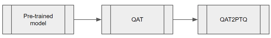
 Ray and path tracing algorithms construct light paths by starting at the camera or the light sources and intersecting rays with the scene geometry. As objects…
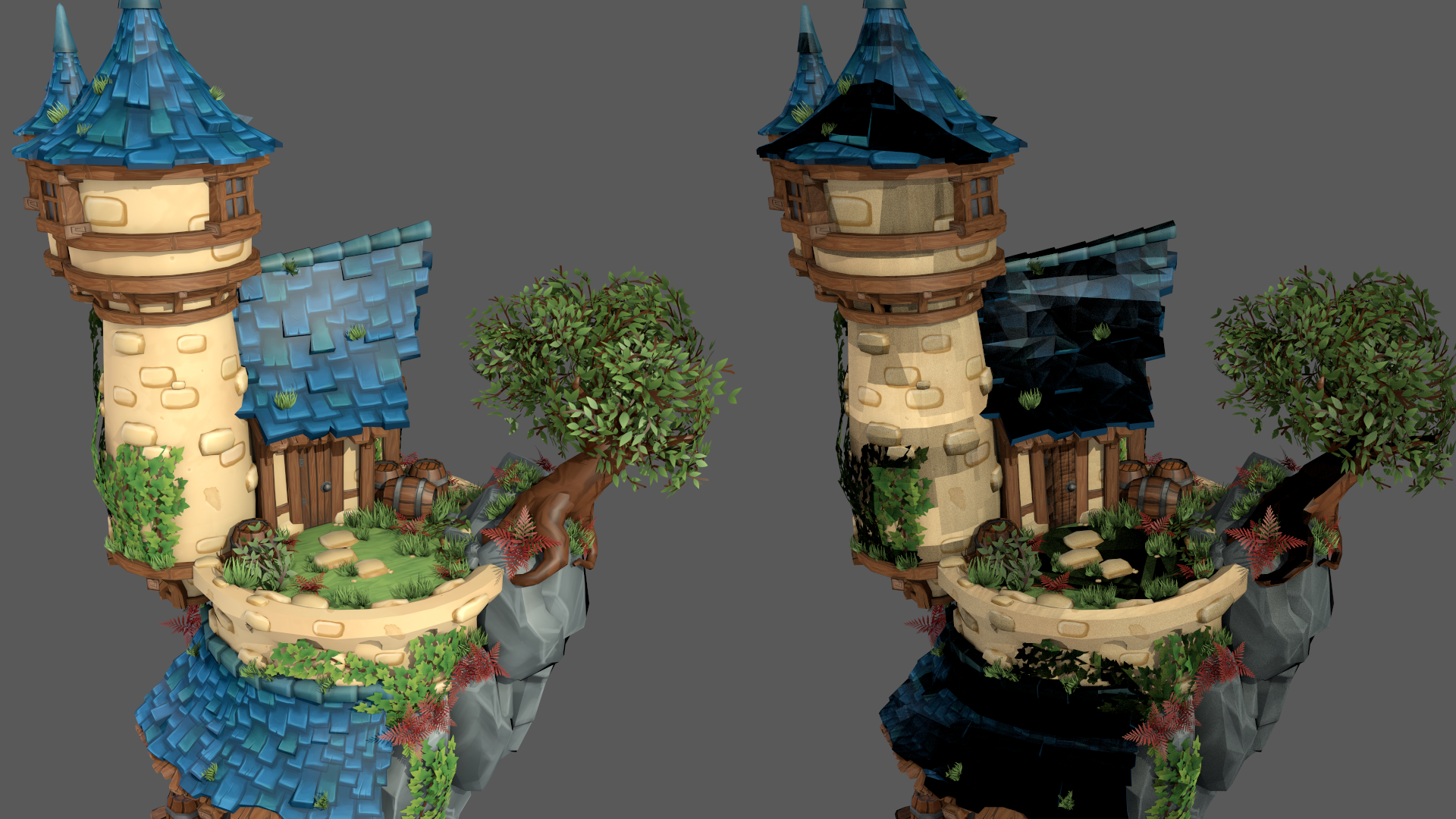
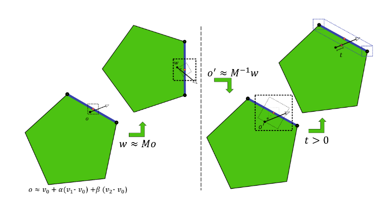
 of the transformation is added last. This again reduces the rounding error on the translation, which in practice tends to dominate the error in this computation.

 from Listing 3. The world-space offset
  simplifies to
  . The object-space offset
  along the object-space normal
  needs to be transformed into world-space as
  .
.  . To obtain a single combined offset along the world-space normal, project the transformed object-space offset onto the world-space normal, as
  . Using that
  this simplifies to:
 from the scene origin in world-space will have a maximum rounding error in the order of
  , or 1 mm of offset for every 4 km distance. The offset magnitudes also scale linear with the triangle extent and object-space position.
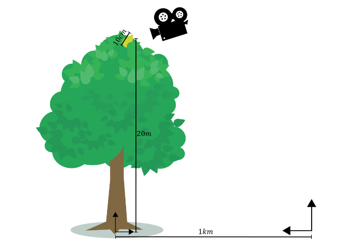
 Graph neural networks (GNNs) have emerged as a powerful tool for a variety of machine learning tasks on graph-structured data. These tasks range from node…
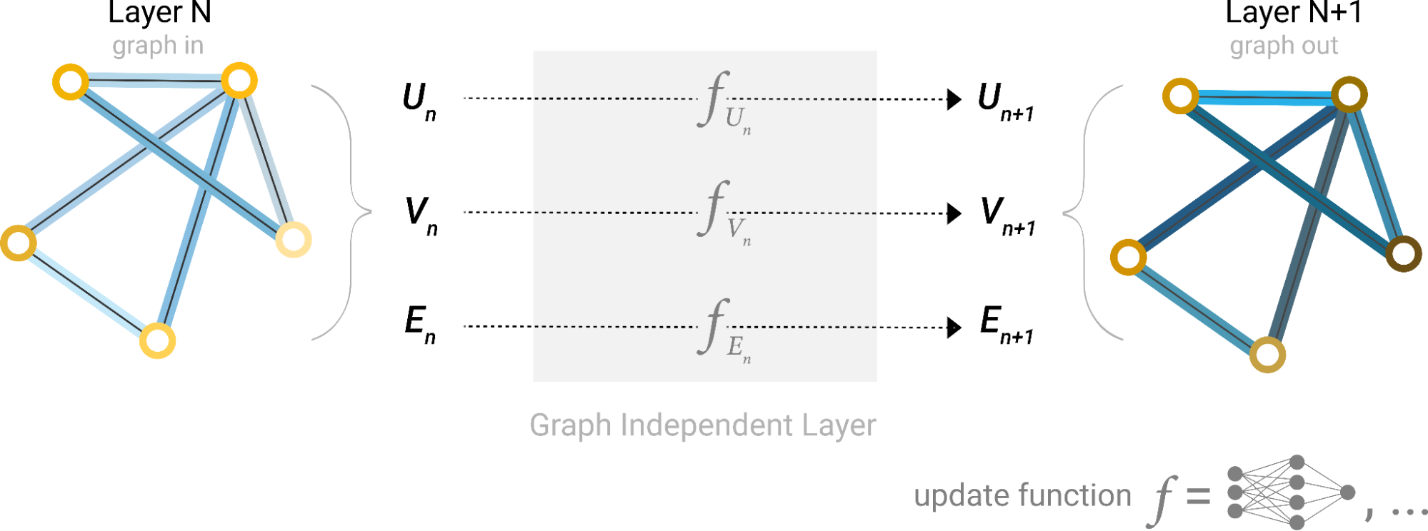
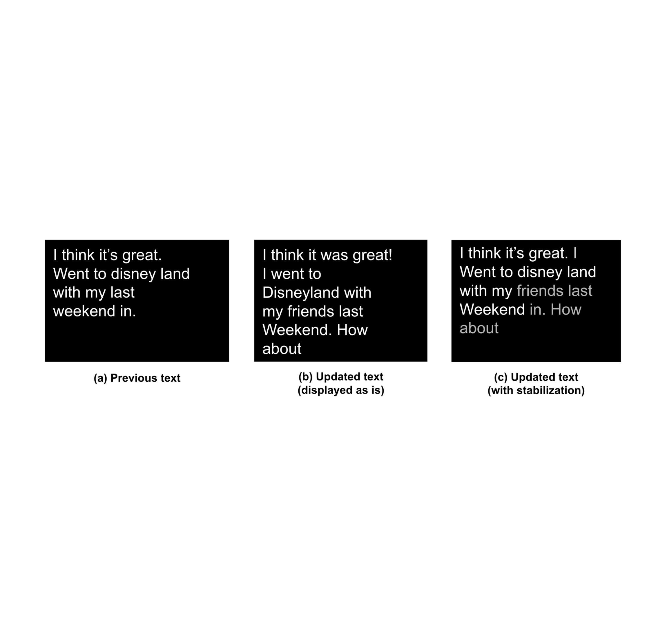


 Caching is as fundamental to computing as arrays, symbols, or strings. Various layers of caching throughout the stack hold instructions from memory while…
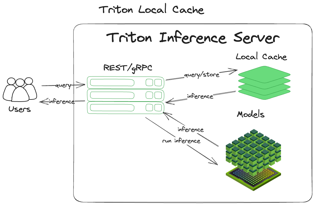
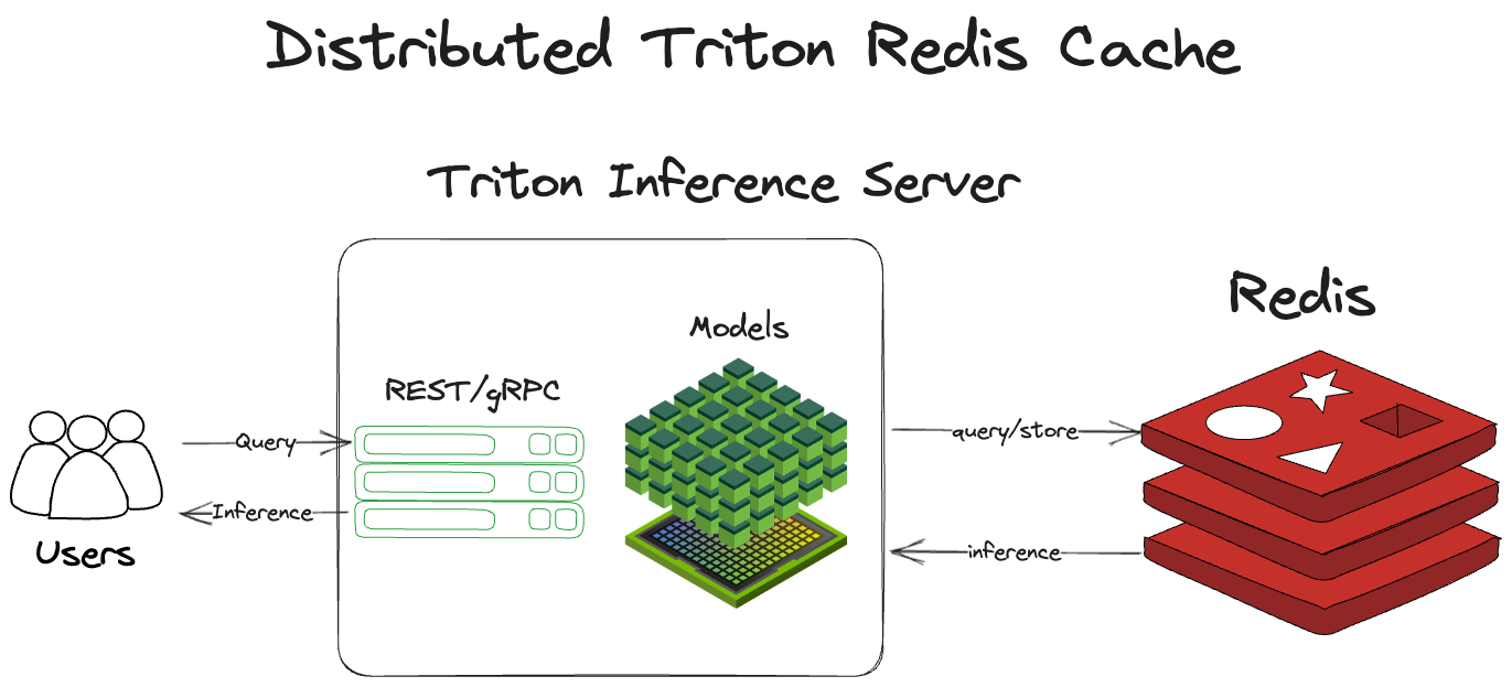
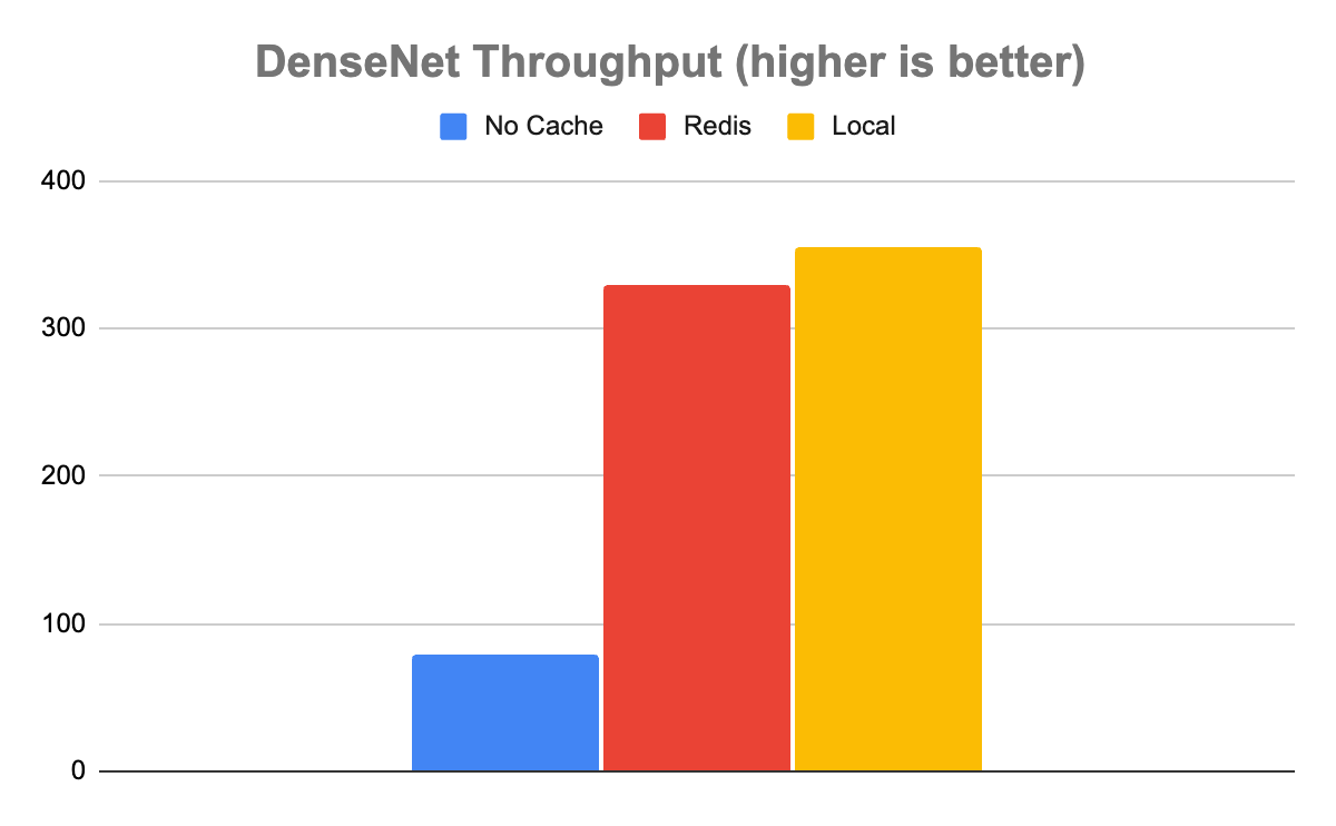
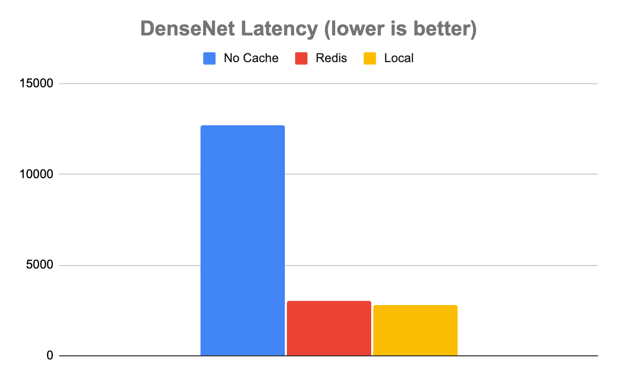
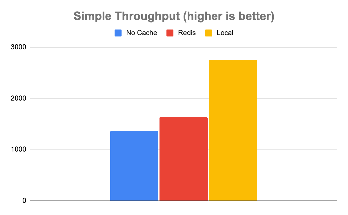
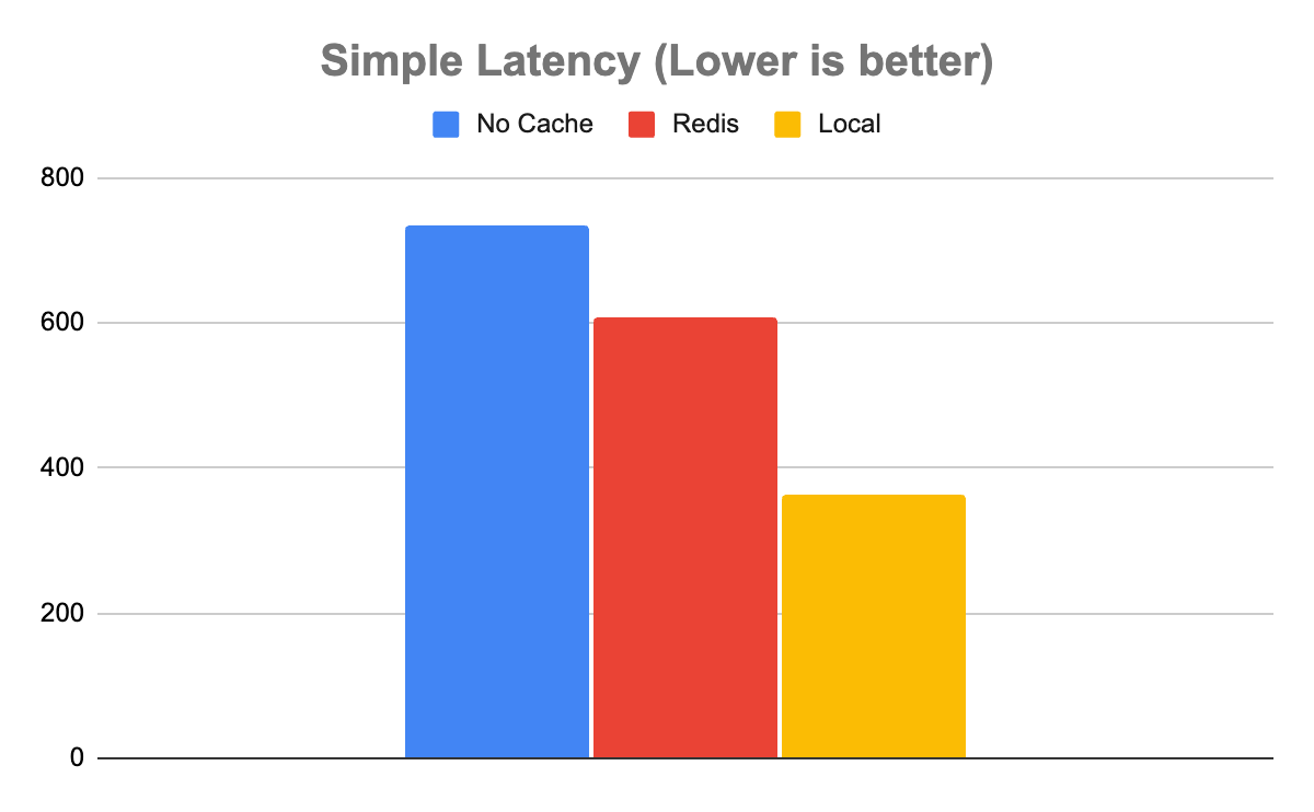
 Learn to create an end-to-end machine learning pipeline for large datasets with this virtual, hands-on workshop.