Category: Offsites

Posted by Boris Babenko, Software Engineer and Naama Hammel, Clinical Research Scientist, Google Health

Three years ago we wrote about our work on predicting a number of cardiovascular risk factors from fundus photos (i.e., photos of the back of the eye)¹ using deep learning. That such risk factors could be extracted from fundus photos was a novel discovery and thus a surprising outcome to clinicians and laypersons alike. Since then, we and other researchers have discovered additional novel biomarkers from fundus photos, such as markers for chronic kidney disease and diabetes, and hemoglobin levels to detect anemia.

A unifying goal of work like this is to develop new disease detection or monitoring approaches that are less invasive, more accurate, cheaper and more readily available. However, one restriction to potential broad population-level applicability of efforts to extract biomarkers from fundus photos is getting the fundus photos themselves, which requires specialized imaging equipment and a trained technician.

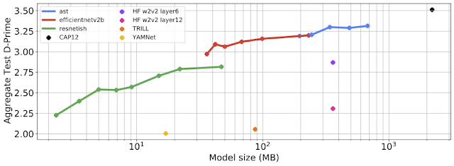
The eye can be imaged in multiple ways. A common approach for diabetic retinal disease screening is to examine the posterior segment using fundus photographs (left), which have been shown to contain signals of kidney and heart disease, as well as anemia. Another way is to take photographs of the front of the eye (external eye photos; right), which is typically used to track conditions affecting the eyelids, conjunctiva, cornea, and lens.

In “Detection of signs of disease in external photographs of the eyes via deep learning”, in press at Nature Biomedical Engineering, we show that a deep learning model can extract potentially useful biomarkers from external eye photos (i.e., photos of the front of the eye). In particular, for diabetic patients, the model can predict the presence of diabetic retinal disease, elevated HbA1c (a biomarker of diabetic blood sugar control and outcomes), and elevated blood lipids (a biomarker of cardiovascular risk). External eye photos as an imaging modality are particularly interesting because their use may reduce the need for specialized equipment, opening the door to various avenues of improving the accessibility of health screening.

Developing the Model
To develop the model, we used de-identified data from over 145,000 patients from a teleretinal diabetic retinopathy screening program. We trained a convolutional neural network both on these images and on the corresponding ground truth for the variables we wanted the model to predict (i.e., whether the patient has diabetic retinal disease, elevated HbA1c, or elevated lipids) so that the neural network could learn from these examples. After training, the model is able to take external eye photos as input and then output predictions for whether the patient has diabetic retinal disease, or elevated sugars or lipids.

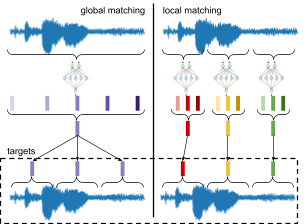
A schematic showing the model generating predictions for an external eye photo.

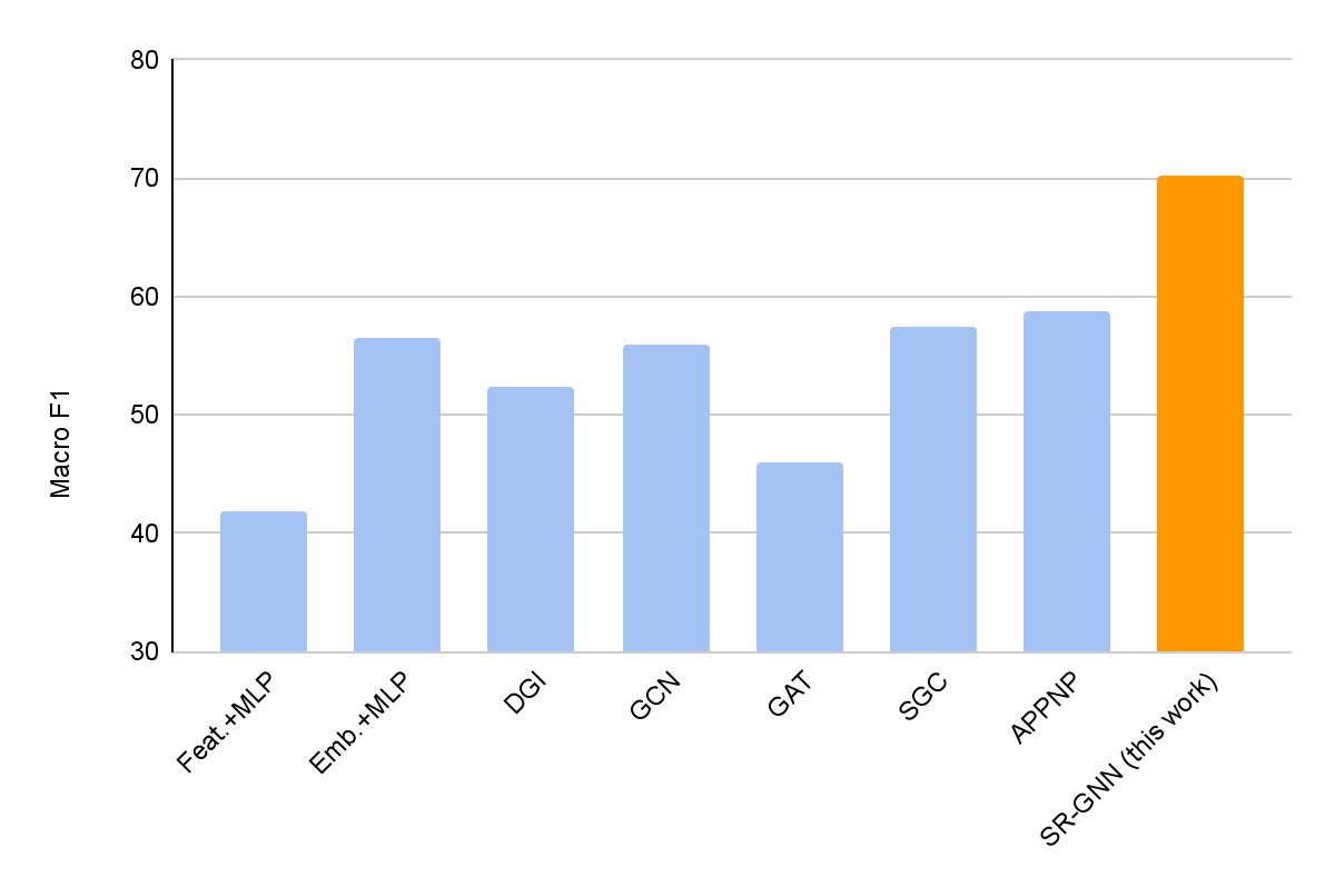
We measured model performance using the area under the receiver operator characteristic curve (AUC), which quantifies how frequently the model assigns higher scores to patients who are truly positive than patients who are truly negative (i.e., a perfect model scores 100%, compared to 50% for random guesses). The model detected various forms of diabetic retinal disease with AUCs of 71-82%, AUCs of 67-70% for elevated HbA1c, and AUCs of 57-68% for elevated lipids. These results indicate that, though imperfect, external eye photos can help detect and quantify various parameters of systemic health.

Much like the CDC’s pre-diabetes screening questionnaire, external eye photos may be able to help “pre-screen” people and identify those who may benefit from further confirmatory testing. If we sort all patients in our study based on their predicted risk and look at the top 5% of that list, 69% of those patients had HbA1c measurements ≥ 9 (indicating poor blood sugar control for patients with diabetes). For comparison, among patients who are at highest risk according to a risk score based on demographics and years with diabetes, only 55% had HbA1c ≥ 9, and among patients selected at random only 33% had HbA1c ≥ 9.

Assessing Potential Bias
We emphasize that this is promising, yet early, proof-of-concept research showcasing a novel discovery. That said, because we believe that it is important to evaluate potential biases in the data and model, we undertook a multi-pronged approach for bias assessment.

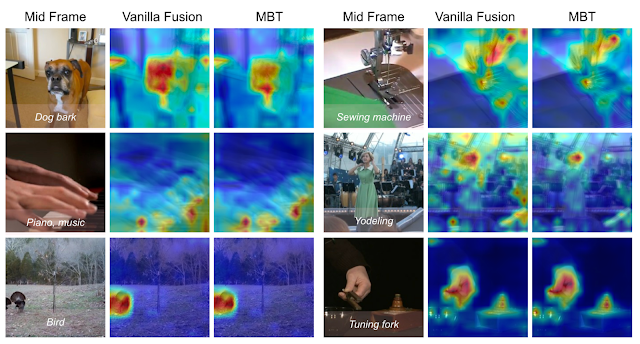
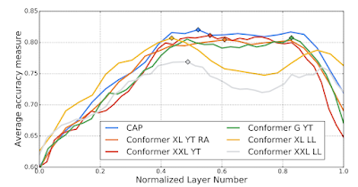
First, we conducted various explainability analyses aimed at discovering what parts of the image contribute most to the algorithm’s predictions (similar to our anemia work). Both saliency analyses (which examine which pixels most influenced the predictions) and ablation experiments (which examine the impact of removing various image regions) indicate that the algorithm is most influenced by the center of the image (the areas of the sclera, iris, and pupil of the eye, but not the eyelids). This is demonstrated below where one can see that the AUC declines much more quickly when image occlusion starts in the center (green lines) than when it starts in the periphery (blue lines).

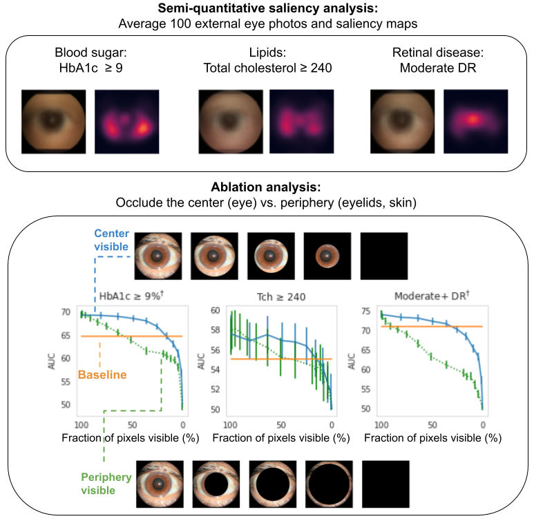
Explainability analysis shows that (top) all predictions focused on different parts of the eye, and that (bottom) occluding the center of the image (corresponding to parts of the eyeball) has a much greater effect than occluding the periphery (corresponding to the surrounding structures, such as eyelids), as shown by the green line’s steeper decline. The “baseline” is a logistic regression model that takes self-reported age, sex, race and years with diabetes as input.

Second, our development dataset spanned a diverse set of locations within the U.S., encompassing over 300,000 de-identified photos taken at 301 diabetic retinopathy screening sites. Our evaluation datasets comprised over 95,000 images from 198 sites in 18 US states, including datasets of predominantly Hispanic or Latino patients, a dataset of majority Black patients, and a dataset that included patients without diabetes. We conducted extensive subgroup analyses across groups of patients with different demographic and physical characteristics (such as age, sex, race and ethnicity, presence of cataract, pupil size, and even camera type), and controlled for these variables as covariates. The algorithm was more predictive than the baseline in all subgroups after accounting for these factors.

Conclusion
This exciting work demonstrates the feasibility of extracting useful health related signals from external eye photographs, and has potential implications for the large and rapidly growing population of patients with diabetes or other chronic diseases. There is a long way to go to achieve broad applicability, for example understanding what level of image quality is needed, generalizing to patients with and without known chronic diseases, and understanding generalization to images taken with different cameras and under a wider variety of conditions, like lighting and environment. In continued partnership with academic and nonacademic experts, including EyePACS and CGMH, we look forward to further developing and testing our algorithm on larger and more comprehensive datasets, and broadening the set of biomarkers recognized (e.g., for liver disease). Ultimately we are working towards making non-invasive health and wellness tools more accessible to everyone.

Acknowledgements
This work involved the efforts of a multidisciplinary team of software engineers, researchers, clinicians and cross functional contributors. Key contributors to this project include: Boris Babenko, Akinori Mitani, Ilana Traynis, Naho Kitade‎, Preeti Singh, April Y. Maa, Jorge Cuadros, Greg S. Corrado, Lily Peng, Dale R. Webster, Avinash Varadarajan‎, Naama Hammel, and Yun Liu. The authors would also like to acknowledge Huy Doan, Quang Duong, Roy Lee, and the Google Health team for software infrastructure support and data collection. We also thank Tiffany Guo, Mike McConnell, Michael Howell, and Sam Kavusi for their feedback on the manuscript. Last but not least, gratitude goes to the graders who labeled data for the pupil segmentation model, and a special thanks to Tom Small for the ideation and design that inspired the animation used in this blog post.

---

¹The information presented here is research and does not reflect a product that is available for sale. Future availability cannot be guaranteed. ^↩

Posted by Mohammad Saleh, Software Engineer, Google Research, Brain Team and Anjuli Kannan, Software Engineer, Google Docs

For many of us, it can be challenging to keep up with the volume of documents that arrive in our inboxes every day: reports, reviews, briefs, policies and the list goes on. When a new document is received, readers often wish it included a brief summary of the main points in order to effectively prioritize it. However, composing a document summary can be cognitively challenging and time-consuming, especially when a document writer is starting from scratch.

To help with this, we recently announced that Google Docs now automatically generates suggestions to aid document writers in creating content summaries, when they are available. Today we describe how this was enabled using a machine learning (ML) model that comprehends document text and, when confident, generates a 1-2 sentence natural language description of the document content. However, the document writer maintains full control — accepting the suggestion as-is, making necessary edits to better capture the document summary or ignoring the suggestion altogether. Readers can also use this section, along with the outline, to understand and navigate the document at a high level. While all users can add summaries, auto-generated suggestions are currently only available to Google Workspace business customers. Building on grammar suggestions, Smart Compose, and autocorrect, we see this as another valuable step toward improving written communication in the workplace.

A blue summary icon appears in the top left corner when a document summary suggestion is available. Document writers can then view, edit, or ignore the suggested document summary.

Model Details
Automatically generated summaries would not be possible without the tremendous advances in ML for natural language understanding (NLU) and natural language generation (NLG) over the past five years, especially with the introduction of Transformer and Pegasus.

Abstractive text summarization, which combines the individually challenging tasks of long document language understanding and generation, has been a long-standing problem in NLU and NLG research. A popular method for combining NLU and NLG is training an ML model using sequence-to-sequence learning, where the inputs are the document words, and the outputs are the summary words. A neural network then learns to map input tokens to output tokens. Early applications of the sequence-to-sequence paradigm used recurrent neural networks (RNNs) for both the encoder and decoder.

The introduction of Transformers provided a promising alternative to RNNs because Transformers use self-attention to provide better modeling of long input and output dependencies, which is critical in document summarization. Still, these models require large amounts of manually labeled data to train sufficiently, so the advent of Transformers alone was not enough to significantly advance the state-of-the-art in document summarization.

The combination of Transformers with self-supervised pre-training (e.g., BERT, GPT, T5) led to a major breakthrough in many NLU tasks for which limited labeled data is available. In self-supervised pre-training, a model uses large amounts of unlabeled text to learn general language understanding and generation capabilities. Then, in a subsequent fine-tuning stage, the model learns to apply these abilities on a specific task, such as summarization or question answering.

The Pegasus work took this idea one step further, by introducing a pre-training objective customized to abstractive summarization. In Pegasus pre-training, also called Gap Sentence Prediction (GSP), full sentences from unlabeled news articles and web documents are masked from the input and the model is required to reconstruct them, conditioned on the remaining unmasked sentences. In particular, GSP attempts to mask sentences that are considered essential to the document through different heuristics. The intuition is to make the pre-training as close as possible to the summarization task. Pegasus achieved state-of-the-art results on a varied set of summarization datasets. However, a number of challenges remained to apply this research advancement into a product.

Applying Recent Research Advances to Google Docs

• Data

  Self-supervised pre-training results in an ML model that has general language understanding and generation capabilities, but a subsequent fine-tuning stage is critical for the model to adapt to the application domain. We fine-tuned early versions of our model on a corpus of documents with manually-generated summaries that were consistent with typical use cases.

  However, early versions of this corpus suffered from inconsistencies and high variation because they included many types of documents, as well as many ways to write a summary — e.g., academic abstracts are typically long and detailed, while executive summaries are brief and punchy. This led to a model that was easily confused because it had been trained on so many different types of documents and summaries that it struggled to learn the relationships between any of them.

  Fortunately, one of the key findings in the Pegasus work was that an effective pre-training phase required less supervised data in the fine-tuning stage. Some summarization benchmarks required as few as 1,000 fine-tuning examples for Pegasus to match the performance of Transformer baselines that saw 10,000+ supervised examples — suggesting that one could focus on quality rather than quantity.

  We carefully cleaned and filtered the fine-tuning data to contain training examples that were more consistent and represented a coherent definition of summaries. Despite the fact that we reduced the amount of training data, this led to a higher quality model. The key lesson, consistent with recent work in domains like dataset distillation, was that it was better to have a smaller, high quality dataset, than a larger, high-variance dataset.

• Serving

  Once we trained the high quality model, we turned to the challenge of serving the model in production. While the Transformer version of the encoder-decoder architecture is the dominant approach to train models for sequence-to-sequence tasks like abstractive summarization, it can be inefficient and impractical to serve in real-world applications. The main inefficiency comes from the Transformer decoder where we generate the output summary token by token through autoregressive decoding. The decoding process becomes noticeably slow when summaries get longer since the decoder attends to all previously generated tokens at each step. RNNs are a more efficient architecture for decoding since there is no self-attention with previous tokens as in a Transformer model.

  We used knowledge distillation, which is the process of transferring knowledge from a large model to a smaller more efficient model, to distill the Pegasus model into a hybrid architecture of a Transformer encoder and an RNN decoder. To improve efficiency we also reduced the number of RNN decoder layers. The resulting model had significant improvements in latency and memory footprint while the quality was still on par with the original model. To further improve the latency and user experience, we serve the summarization model using TPUs, which provide significant speed ups and allow more requests to be handled by a single machine.

Ongoing Challenges and Next Steps
While we are excited by the progress so far, there are a few challenges we are continuing to tackle:

• Document coverage: Developing a set of documents for the fine-tuning stage was difficult due to the tremendous variety that exists among documents, and the same challenge is true at inference time. Some of the documents our users create (e.g., meeting notes, recipes, lesson plans and resumes) are not suitable for summarization or can be difficult to summarize. Currently, our model only suggests a summary for documents where it is most confident, but we hope to continue broadening this set as our model improves.
• Evaluation: Abstractive summaries need to capture the essence of a document while being fluent and grammatically correct. A specific document may have many summaries that can be considered correct, and different readers may prefer different ones. This makes it hard to evaluate summaries with automatic metrics only, user feedback and usage statistics will be critical for us to understand and keep improving quality.
• Long documents: Long documents are some of the toughest documents for the model to summarize because it is harder to capture all the points and abstract them in a single summary, and it can also significantly increase memory usage during training and serving. However, long documents are perhaps most useful for the model to automatically summarize because it can help document writers get a head start on this tedious task. We hope we can apply the latest ML advancements to better address this challenge.

Conclusion
Overall, we are thrilled that we can apply recent progress in NLU and NLG to continue assisting users with reading and writing. We hope the automatic suggestions now offered in Google Workspace make it easier for writers to annotate their documents with summaries, and help readers comprehend and navigate documents more easily.

Acknowledgements
The authors would like to thank the many people across Google that contributed to this work: AJ Motika, Matt Pearson-Beck, Mia Chen, Mahdis Mahdieh, Halit Erdogan, Benjamin Lee, Ali Abdelhadi, Michelle Danoff, Vishnu Sivaji, Sneha Keshav, Aliya Baptista, Karishma Damani, DJ Lick, Yao Zhao, Peter Liu, Aurko Roy, Yonghui Wu, Shubhi Sareen, Andrew Dai, Mekhola Mukherjee, Yinan Wang, Mike Colagrosso, and Behnoosh Hariri. .

Posted by Amir Yazdanbakhsh, Research Scientist and Aviral Kumar, Student Researcher, Google Research

Advances in machine learning (ML) often come with advances in hardware and computing systems. For example, the growth of ML-based approaches in solving various problems in vision and language has led to the development of application-specific hardware accelerators (e.g., Google TPUs and Edge TPUs). While promising, standard procedures for designing accelerators customized towards a target application require manual effort to devise a reasonably accurate simulator of hardware, followed by performing many time-intensive simulations to optimize the desired objective (e.g., optimizing for low power usage or latency when running a particular application). This involves identifying the right balance between total amount of compute and memory resources and communication bandwidth under various design constraints, such as the requirement to meet an upper bound on chip area usage and peak power. However, designing accelerators that meet these design constraints is often result in infeasible designs. To address these challenges, we ask: “Is it possible to train an expressive deep neural network model on large amounts of existing accelerator data and then use the learned model to architect future generations of specialized accelerators, eliminating the need for computationally expensive hardware simulations?”

In “Data-Driven Offline Optimization for Architecting Hardware Accelerators”, accepted at ICLR 2022, we introduce PRIME, an approach focused on architecting accelerators based on data-driven optimization that only utilizes existing logged data (e.g., data leftover from traditional accelerator design efforts), consisting of accelerator designs and their corresponding performance metrics (e.g., latency, power, etc) to architect hardware accelerators without any further hardware simulation. This alleviates the need to run time-consuming simulations and enables reuse of data from past experiments, even when the set of target applications changes (e.g., an ML model for vision, language, or other objective), and even for unseen but related applications to the training set, in a zero-shot fashion. PRIME can be trained on data from prior simulations, a database of actually fabricated accelerators, and also a database of infeasible or failed accelerator designs¹. This approach for architecting accelerators — tailored towards both single- and multi-applications — improves performance upon state-of-the-art simulation-driven methods by about 1.2x-1.5x, while considerably reducing the required total simulation time by 93% and 99%, respectively. PRIME also architects effective accelerators for unseen applications in a zero-shot setting, outperforming simulation-based methods by 1.26x.

PRIME uses logged accelerator data, consisting of both feasible and infeasible accelerators, to train a conservative model, which is used to design accelerators while meeting design constraints. PRIME architects accelerators with up to 1.5x smaller latency, while reducing the required hardware simulation time by up to 99%.

The PRIME Approach for Architecting Accelerators
Perhaps the simplest possible way to use a database of previously designed accelerators for hardware design is to use supervised machine learning to train a prediction model that can predict the performance objective for a given accelerator as input. Then, one could potentially design new accelerators by optimizing the performance output of this learned model with respect to the input accelerator design. Such an approach is known as model-based optimization. However, this simple approach has a key limitation: it assumes that the prediction model can accurately predict the cost for every accelerator that we might encounter during optimization! It is well established that most prediction models trained via supervised learning misclassify adversarial examples that “fool” the learned model into predicting incorrect values. Similarly, it has been shown that even optimizing the output of a supervised model finds adversarial examples that look promising under the learned model², but perform terribly under the ground truth objective.

To address this limitation, PRIME learns a robust prediction model that is not prone to being fooled by adversarial examples (that we will describe shortly), which would be otherwise found during optimization. One can then simply optimize this model using any standard optimizer to architect simulators. More importantly, unlike prior methods, PRIME can also utilize existing databases of infeasible accelerators to learn what not to design. This is done by augmenting the supervised training of the learned model with additional loss terms that specifically penalize the value of the learned model on the infeasible accelerator designs and adversarial examples during training. This approach resembles a form of adversarial training.

In principle, one of the central benefits of a data-driven approach is that it should enable learning highly expressive and generalist models of the optimization objective that generalize over target applications, while also potentially being effective for new unseen applications for which a designer has never attempted to optimize accelerators. To train PRIME so that it generalizes to unseen applications, we modify the learned model to be conditioned on a context vector that identifies a given neural net application we wish to accelerate (as we discuss in our experiments below, we choose to use high-level features of the target application: such as number of feed-forward layers, number of convolutional layers, total parameters, etc. to serve as the context), and train a single, large model on accelerator data for all applications designers have seen so far. As we will discuss below in our results, this contextual modification of PRIME enables it to optimize accelerators both for multiple, simultaneous applications and new unseen applications in a zero-shot fashion.

Does PRIME Outperform Custom-Engineered Accelerators?
We evaluate PRIME on a variety of actual accelerator design tasks. We start by comparing the optimized accelerator design architected by PRIME targeted towards nine applications to the manually optimized EdgeTPU design. EdgeTPU accelerators are primarily optimized towards running applications in image classification, particularly MobileNetV2, MobileNetV3 and MobileNetEdge. Our goal is to check if PRIME can design an accelerator that attains a lower latency than a baseline EdgeTPU accelerator³, while also constraining the chip area to be under 27 mm² (the default for the EdgeTPU accelerator). Shown below, we find that PRIME improves latency over EdgeTPU by 2.69x (up to 11.84x in t-RNN Enc), while also reducing the chip area usage by 1.50x (up to 2.28x in MobileNetV3), even though it was never trained to reduce chip area! Even on the MobileNet image-classification models, for which the custom-engineered EdgeTPU accelerator was optimized, PRIME improves latency by 1.85x.

Comparing latencies (lower is better) of accelerator designs suggested by PRIME and EdgeTPU for single-model specialization.

The chip area (lower is better) reduction compared to a baseline EdgeTPU design for single-model specialization.

Designing Accelerators for New and Multiple Applications, Zero-Shot
We now study how PRIME can use logged accelerator data to design accelerators for (1) multiple applications, where we optimize PRIME to design a single accelerator that works well across multiple applications simultaneously, and in a (2) zero-shot setting, where PRIME must generate an accelerator for new unseen application(s) without training on any data from such applications. In both settings, we train the contextual version of PRIME, conditioned on context vectors identifying the target applications and then optimize the learned model to obtain the final accelerator. We find that PRIME outperforms the best simulator-driven approach in both settings, even when very limited data is provided for training for a given application but many applications are available. Specifically in the zero-shot setting, PRIME outperforms the best simulator-driven method we compared to, attaining a reduction of 1.26x in latency. Further, the difference in performance increases as the number of training applications increases.

The average latency (lower is better) of test applications under zero-shot setting compared to a state-of-the-art simulator-driven approach. The text on top of each bar shows the set of training applications.

Closely Analyzing an Accelerator Designed by PRIME
To provide more insight to hardware architecture, we examine the best accelerator designed by PRIME and compare it to the best accelerator found by the simulator-driven approach. We consider the setting where we need to jointly optimize the accelerator for all nine applications, MobileNetEdge, MobileNetV2, MobileNetV3, M4, M5, M6⁴, t-RNN Dec, and t-RNN Enc, and U-Net, under a chip area constraint of 100 mm². We find that PRIME improves latency by 1.35x over the simulator-driven approach.

Per application latency (lower is better) for the best accelerator design suggested by PRIME and state-of-the-art simulator-driven approach for a multi-task accelerator design. PRIME reduces the average latency across all nine applications by 1.35x over the simulator-driven method.

As shown above, while the latency of the accelerator designed by PRIME for MobileNetEdge, MobileNetV2, MobileNetV3, M4, t-RNN Dec, and t-RNN Enc are better, the accelerator found by the simulation-driven approach yields a lower latency in M5, M6, and U-Net. By closely inspecting the accelerator configurations, we find that PRIME trades compute (64 cores for PRIME vs. 128 cores for the simulator-driven approach) for larger Processing Element (PE) memory size (2,097,152 bytes vs. 1,048,576 bytes). These results show that PRIME favors PE memory size to accommodate the larger memory requirements in t-RNN Dec and t-RNN Enc, where large reductions in latency were possible. Under a fixed area budget, favoring larger on-chip memory comes at the expense of lower compute power in the accelerator. This reduction in the accelerator’s compute power leads to higher latency for the models with large numbers of compute operations, namely M5, M6, and U-Net.

Conclusion
The efficacy of PRIME highlights the potential for utilizing the logged offline data in an accelerator design pipeline. A likely avenue for future work is to scale this approach across an array of applications, where we expect to see larger gains because simulator-driven approaches would need to solve a complex optimization problem, akin to searching for needle in a haystack, whereas PRIME can benefit from generalization of the surrogate model. On the other hand, we would also note that PRIME outperforms prior simulator-driven methods we utilize and this makes it a promising candidate to be used within a simulator-driven method. More generally, training a strong offline optimization algorithm on offline datasets of low-performing designs can be a highly effective ingredient in at the very least, kickstarting hardware design, versus throwing out prior data. Finally, given the generality of PRIME, we hope to use it for hardware-software co-design, which exhibits a large search space but plenty of opportunity for generalization. We have also released both the code for training PRIME and the dataset of accelerators.

Acknowledgments
We thank our co-authors Sergey Levine, Kevin Swersky, and Milad Hashemi for their advice, thoughts and suggestions. We thank James Laudon, Cliff Young, Ravi Narayanaswami, Berkin Akin, Sheng-Chun Kao, Samira Khan, Suvinay Subramanian, Stella Aslibekyan, Christof Angermueller, and Olga Wichrowskafor for their help and support, and Sergey Levine for feedback on this blog post. In addition, we would like to extend our gratitude to the members of “Learn to Design Accelerators”, “EdgeTPU”, and the Vizier team for providing invaluable feedback and suggestions. We would also like to thank Tom Small for the animated figure used in this post.

---

¹The infeasible accelerator designs stem from build errors in silicon or compilation/mapping failures. ^↩
2This is akin to adversarial examples in supervised learning – these examples are close to the data points observed in the training dataset, but are misclassified by the classifier. ^↩
3The performance metrics for the baseline EdgeTPU accelerator are extracted from an industry-based hardware simulator tuned to match the performance of the actual hardware. ^↩
4These are proprietary object-detection models, and we refer to them as M4 (indicating Model 4), M5, and M6 in the paper. ^↩

Posted by William J. Huggins, Research Scientist, Google Quantum AI

The intersection between the computational difficulty and practical importance of quantum chemistry challenges run on quantum computers has long been a focus for Google Quantum AI. We’ve experimentally simulated simple models of chemical bonding, high-temperature superconductivity, nanowires, and even exotic phases of matter such as time crystals on our Sycamore quantum processors. We’ve also developed algorithms suitable for the error-corrected quantum computers we aim to build, including the world’s most efficient algorithm for large-scale quantum computations of chemistry (in the usual way of formulating the problem) and a pioneering approach that allows for us to solve the same problem at an extremely high spatial resolution by encoding the position of the electrons differently.

Despite these successes, it is still more effective to use classical algorithms for studying quantum chemistry than the noisy quantum processors we have available today. However, when the laws of quantum mechanics are translated into programs that a classical computer can run, we often find that the amount of time or memory required scales very poorly with the size of the physical system to simulate.

Today, in collaboration with Dr. Joonho Lee and Professor David Reichmann at Colombia, we present the Nature publication “Unbiasing Fermionic Quantum Monte Carlo with a Quantum Computer”, where we propose and experimentally validate a new way of combining classical and quantum computation to study chemistry, which can replace a computationally-expensive subroutine in a powerful classical algorithm with a “cheaper”, noisy, calculation on a small quantum computer. To evaluate the performance of this hybrid quantum-classical approach, we applied this idea to perform the largest quantum computation of chemistry to date, using 16 qubits to study the forces experienced by two carbon atoms in a diamond crystal. Not only was this experiment four qubits larger than our earlier chemistry calculations on Sycamore, we were also able to use a more comprehensive description of the physics that fully incorporated the interactions between electrons.

Google’s Sycamore quantum processor. Photo Credit: Rocco Ceselin.

A New Way of Combining Quantum and Classical
Our starting point was to use a family of Monte Carlo techniques (projector Monte Carlo, more on that below) to give us a useful description of the lowest energy state of a quantum mechanical system (like the two carbon atoms in a crystal mentioned above). However, even just storing a good description of a quantum state (the “wavefunction”) on a classical computer can be prohibitively expensive, let alone calculating one.

Projector Monte Carlo methods provide a way around this difficulty. Instead of writing down a full description of the state, we design a set of rules for generating a large number of oversimplified descriptions of the state (for example, lists of where each electron might be in space) whose average is a good approximation to the real ground state. The “projector” in projector Monte Carlo refers to how we design these rules — by continuously trying to filter out the incorrect answers using a mathematical process called projection, similar to how a silhouette is a projection of a three-dimensional object onto a two-dimensional surface.

Unfortunately, when it comes to chemistry or materials science, this idea isn’t enough to find the ground state on its own. Electrons belong to a class of particles known as fermions, which have a surprising quantum mechanical quirk to their behavior. When two identical fermions swap places, the quantum mechanical wavefunction (the mathematical description that tells us everything there is to know about them) picks up a minus sign. This minus sign gives rise to the famous Pauli exclusion principle (the fact that two fermions cannot occupy the same state). It can also cause projector Monte Carlo calculations to become inefficient or even break down completely. The usual resolution to this fermion sign problem involves tweaking the Monte Carlo algorithm to include some information from an approximation to the ground state. By using an approximation (even a crude one) to the lowest energy state as a guide, it is usually possible to avoid breakdowns and even obtain accurate estimates of the properties of the true ground state.

Top: An illustration of how the fermion sign problem appears in some cases. Instead of following the blue line curve, our estimates of the energy follow the red curve and become unstable. Bottom: An example of the improvements we might see when we try to fix the sign problem. By using a quantum computer, we hope to improve the initial guess that guides our calculation and obtain a more accurate answer.

For the most challenging problems (such as modeling the breaking of chemical bonds), the computational cost of using an accurate enough initial guess on a classical computer can be too steep to afford, which led our collaborator Dr. Joonho Lee to ask if a quantum computer could help. We had already demonstrated in previous experiments that we can use our quantum computer to approximate the ground state of a quantum system. In these earlier experiments we aimed to measure quantities (such as the energy of the state) that are directly linked to physical properties (like the rate of a chemical reaction). In this new hybrid algorithm, we instead needed to make a very different kind of measurement: quantifying how far the states generated by the Monte Carlo algorithm on our classical computer are from those prepared on the quantum computer. Using some recently developed techniques, we were even able to do all of the measurements on the quantum computer before we ran the Monte Carlo algorithm, separating the quantum computer’s job from the classical computer’s.

A diagram of our calculation. The quantum processor (right) measures information that guides the classical calculation (left). The crosses indicate the qubits, with the ones used for the largest experiment shaded green. The direction of the arrows indicate that the quantum processor doesn’t need any feedback from the classical calculation. The red bars represent the parts of the classical calculation that are filtered out by the data from the quantum computer in order to avoid the fermion sign problem and get a good estimate of properties like the energy of the ground state.

This division of labor between the classical and the quantum computer helped us make good use of both resources. Using our Sycamore quantum processor, we prepared a kind of approximation to the ground state that would be difficult to scale up classically. With a few hours of time on the quantum device, we extracted all of the data we needed to run the Monte Carlo algorithm on the classical computer. Even though the data was noisy (like all present-day quantum computations), it had enough signal that it was able to guide the classical computer towards a very accurate reconstruction of the true ground state (shown in the figure below). In fact, we showed that even when we used a low-resolution approximation to the ground state on the quantum computer (just a few qubits encoding the position of the electrons), the classical computer could efficiently solve a much higher resolution version (with more realism about where the electrons can be).

Top left: a diagram showing the sixteen qubits we used for our largest experiment. Bottom left: an illustration of the carbon atoms in a diamond crystal. Our calculation focused on two atoms (the two that are highlighted in translucent yellow). Right: A plot showing how the error in the total energy (closer to zero is better) changes as we adjust the lattice constant (the spacing between the two carbon atoms). Many properties we might care about, such as the structure of the crystal, can be determined by understanding how the energy varies as we move the atoms around. The calculations we performed using the quantum computer (red points) are comparable in accuracy to two state-of-the-art classical methods (yellow and green triangles) and are extremely close to the numbers we would have gotten if we had a perfect quantum computer rather than a noisy one (black points). The fact that these red and black points are so close tells us that the error in our calculation comes from using an approximate ground state on the quantum computer that was too simple, not from being overwhelmed by noise on the device.

Using our new hybrid quantum algorithm, we performed the largest ever quantum computation of chemistry or materials science. We used sixteen qubits to calculate the energy of two carbon atoms in a diamond crystal. This experiment was four qubits larger than our first chemistry calculations on Sycamore, we obtained more accurate results, and we were able to use a better model of the underlying physics. By guiding a powerful classical Monte Carlo calculation using data from our quantum computer, we performed these calculations in a way that was naturally robust to noise.

We’re optimistic about the promise of this new research direction and excited to tackle the challenge of scaling these kinds of calculations up towards the boundary of what we can do with classical computing, and even to the hard-to-study corners of the universe. We know the road ahead of us is long, but we’re excited to have another tool in our growing toolbox.

Acknowledgements
I’d like to thank my co-authors on the manuscript, Bryan O’Gorman, Nicholas Rubin, David Reichman, Ryan Babbush, and especially Joonho Lee for their many contributions, as well as Charles Neill and Pedram Rousham for their help executing the experiment. I’d also like to thank the larger Google Quantum AI team, who designed, built, programmed, and calibrated the Sycamore processor.

Posted by Arsha Nagrani and Chen Sun, Research Scientists, Google Research, Perception Team

People interact with the world through multiple sensory streams (e.g., we see objects, hear sounds, read words, feel textures and taste flavors), combining information and forming associations between senses. As real-world data consists of various signals that co-occur, such as video frames and audio tracks, web images and their captions and instructional videos and speech transcripts, it is natural to apply a similar logic when building and designing multimodal machine learning (ML) models.

Effective multimodal models have wide applications — such as multilingual image retrieval, future action prediction, and vision-language navigation — and are important for several reasons; robustness, which is the ability to perform even when one or more modalities is missing or corrupted, and complementarity between modalities, which is the idea that some information may be present only in one modality (e.g., audio stream) and not in the other (e.g., video frames). While the dominant paradigm for multimodal fusion, called late fusion, consists of using separate models to encode each modality, and then simply combining their output representations at the final step, investigating how to effectively and efficiently combine information from different modalities is still understudied.

In “Attention Bottlenecks for Multimodal Fusion”, published at NeurIPS 2021, we introduce a novel transformer-based model for multimodal fusion in video called Multimodal Bottleneck Transformer (MBT). Our model restricts cross-modal attention flow between latent units in two ways: (1) through tight fusion bottlenecks, that force the model to collect and condense the most relevant inputs in each modality (sharing only necessary information with other modalities), and (2) to later layers of the model, allowing early layers to specialize to information from individual modalities. We demonstrate that this approach achieves state-of-the-art results on video classification tasks, with a 50% reduction in FLOPs compared to a vanilla multimodal transformer model. We have also released our code as a tool for researchers to leverage as they expand on multimodal fusion work.

A Vanilla Multimodal Transformer Model
Transformer models consistently obtain state-of-the-art results in ML tasks, including video (ViViT) and audio classification (AST). Both ViViT and AST are built on the Vision Transformer (ViT); in contrast to standard convolutional approaches that process images pixel-by-pixel, ViT treats an image as a sequence of patch tokens (i.e., tokens from a smaller part, or patch, of an image that is made up of multiple pixels). These models then perform self-attention operations across all pairs of patch tokens. However, using transformers for multimodal fusion is challenging because of their high computational cost, with complexity scaling quadratically with input sequence length.

Because transformers effectively process variable length sequences, the simplest way to extend a unimodal transformer, such as ViT, to the multimodal case is to feed the model a sequence of both visual and auditory tokens, with minimal changes to the transformer architecture. We call this a vanilla multimodal transformer model, which allows free attention flow (called vanilla cross-attention) between different spatial and temporal regions in an image, and across frequency and time in audio inputs, represented by spectrograms. However, while easy to implement by concatenating audio and video input tokens, vanilla cross-attention at all layers of the transformer model is unnecessary because audio and visual inputs contain dense, fine-grained information, which may be redundant for the task — increasing complexity.

Restricting Attention Flow
The issue of growing complexity for long sequences in multimodal models can be mitigated by reducing the attention flow. We restrict attention flow using two methods, specifying the fusion layer and adding attention bottlenecks.

• Fusion layer (early, mid or late fusion): In multimodal models, the layer where cross-modal interactions are introduced is called the fusion layer. The two extreme versions are early fusion (where all layers in the transformer are cross-modal) and late fusion (where all layers are unimodal and no cross-modal information is exchanged in the transformer encoder). Specifying a fusion layer in between leads to mid fusion. This technique builds on a common paradigm in multimodal learning, which is to restrict cross-modal flow to later layers of the network, allowing early layers to specialize in learning and extracting unimodal patterns.
• Attention bottlenecks: We also introduce a small set of latent units that form an attention bottleneck (shown below in purple), which force the model, within a given layer, to collate and condense information from each modality before sharing it with the other, while still allowing free attention flow within a modality. We demonstrate that this bottlenecked version (MBT), outperforms or matches its unrestricted counterpart with lower computational cost.

The different attention configurations in our model. Unlike late fusion (top left), where no cross-modal information is exchanged in the transformer encoder, we investigate two pathways for the exchange of cross-modal information. Early and mid fusion (top middle, top right) is done via standard pairwise self attention across all hidden units in a layer. For mid fusion, cross-modal attention is applied only to later layers in the model. Bottleneck fusion (bottom left) restricts attention flow within a layer through tight latent units called attention bottlenecks. Bottleneck mid fusion (bottom right) applies both forms of restriction in conjunction for optimal performance.

Bottlenecks and Computation Cost
We apply MBT to the task of sound classification using the AudioSet dataset and investigate its performance for two approaches: (1) vanilla cross-attention, and (2) bottleneck fusion. For both approaches, mid fusion (shown by the middle values of the x-axis below) outperforms both early (fusion layer = 0) and late fusion (fusion layer = 12). This suggests that the model benefits from restricting cross-modal connections to later layers, allowing earlier layers to specialize in learning unimodal features; however, it still benefits from multiple layers of cross-modal information flow. We find that adding attention bottlenecks (bottleneck fusion) outperforms or maintains performance with vanilla cross-attention for all fusion layers, with more prominent improvements at lower fusion layers.

The impact of using attention bottlenecks for fusion on mAP performance (left) and compute (right) at different fusion layers on AudioSet. Attention bottlenecks (red) improve performance over vanilla cross-attention (blue) at lower computational cost. Mid fusion, which is in fusion layers 4-10, outperforms both early (fusion layer = 0) and late (fusion layer = 12) fusion, with best performance at fusion layer 8.

We compare the amount of computation, measured in GFLOPs, for both vanilla cross-attention and bottleneck fusion. Using a small number of attention bottlenecks (four bottleneck tokens used in our experiments) adds negligible extra computation over a late fusion model, with computation remaining largely constant with varying fusion layers. This is in contrast to vanilla cross-attention, which has a non-negligible computational cost for every layer it is applied to. We note that for early fusion, bottleneck fusion outperforms vanilla cross-attention by over 2 mean average precision points (mAP) on audiovisual sound classification, with less than half the computational cost.

Results on Sound Classification and Action Recognition
MBT outperforms previous research on popular video classification tasks — sound classification (AudioSet and VGGSound) and action recognition (Kinetics and Epic-Kitchens). For multiple datasets, late fusion and MBT with mid fusion (both fusing audio and vision) outperform the best single modality baseline, and MBT with mid fusion outperforms late fusion.

Across multiple datasets, fusing audio and vision outperforms the best single modality baseline, and MBT with mid fusion outperforms late fusion. For each dataset we report the widely used primary metric, i.e., Audioset: mAP, Epic-Kitchens: Top-1 action accuracy, VGGSound, Moments-in-Time and Kinetics: Top-1 classification accuracy.

Visualization of Attention Heatmaps
To understand the behavior of MBT, we visualize the attention computed by our network following the attention rollout technique. We compute heat maps of the attention from the output classification tokens to the image input space for a vanilla cross-attention model and MBT on the AudioSet test set. For each video clip, we show the original middle frame on the left with the ground truth labels overlayed at the bottom. We demonstrate that the attention is particularly focused on regions in the images that contain motion and create sound, e.g., the fingertips on the piano, the sewing machine, and the face of the dog. The fusion bottlenecks in MBT further force the attention to be localized to smaller regions of the images, e.g., the mouth of the dog in the top left and the woman singing in the middle right. This provides some evidence that the tight bottlenecks force MBT to focus only on the image patches that are relevant for an audio classification task and that benefit from mid fusion with audio.

Summary
We introduce MBT, a new transformer-based architecture for multimodal fusion, and explore various fusion approaches using cross-attention between bottleneck tokens. We demonstrate that restricting cross-modal attention via a small set of fusion bottlenecks achieves state-of-the-art results on a number of video classification benchmarks while also reducing computational costs compared to vanilla cross-attention models.

Acknowledgements
This research was conducted by Arsha Nagrani, Anurag Arnab, Shan Yang, Aren Jansen, Cordelia Schmid and Chen Sun. The blog post was written by Arsha Nagrani, Anurag Arnab and Chen Sun. Animations were created by Tom Small.

Posted by Emily Masten, Software Engineer, Google Research, Operations Research Team

Airlines around the world are exploring several tactics to meet aggressive CO₂ commitments set by the International Civil Aviation Organization (ICAO). This effort has been emphasized in Europe, where aviation accounts for 13.9% of the transportation industry’s carbon emissions. The largest push comes from the European Green Deal, which aims to decrease carbon emissions from transportation by 90% by 2051. The Lufthansa Group has gone even further, committing to a 50% reduction in emissions compared to 2019 by the year 2030 and to reach net-zero emissions by 2050.

One unexpected approach that airlines can use to lower carbon emissions is through optimizing their tail assignment, i.e., how to assign aircraft (identified by the aircraft registration painted on their tails) to legs in a way that minimizes the total operating cost, of which fuel is a major contributor. More fuel needed to operate the aircraft means higher operating costs and more carbon ejected into the atmosphere. For example, a typical long-haul flight (longer than ~4,100km or ~2,500mi) emits about a ton of CO₂.

The amount of fuel needed to fly between origin and destination can vary widely — e.g., larger aircraft weigh more and therefore require more fuel, while modern and younger aircraft tend to be more fuel-efficient because they use newer technology. The mass of the fuel itself is also significant. Aircraft are less fuel-efficient early in their flights when their fuel tanks are full than later when the volume of fuel is reduced. Another important factor for the tail assignment is the number of passengers on board; as the number of bookings changes, a smaller or larger aircraft might be required. Other factors can affect fuel consumption, both negative (e.g., headwinds or the age of the engines) or positive (e.g., tailwinds, sharklets, skin).

During the past year, Google’s Operations Research team has been working with the Lufthansa Group to optimize their tail assignment to reduce carbon emissions and the cost of operating their flights. As part of this collaboration, we developed and launched a mathematical tail assignment solver that has been fully integrated to optimize the fleet schedule for SWISS International Air Lines (a Lufthansa Group subsidiary), which we estimate will result in significant reductions in carbon emissions. This solver is the first step of a multi-phase project that started at SWISS.

A Mathematical Model for Tail Assignment
We structure the task of tail assignment optimization as a network flow problem, which is essentially a directed graph characterized by a set of nodes and a set of arcs, with additional constraints related to the problem at hand. Nodes may have either a supply or a demand for a commodity, while arcs have a flow capacity and a cost per unit of flow. The goal is to determine flows for every arc that minimize the total flow cost of each commodity, while maintaining flow balance in the network.

We decided to use a flow network because it is the most common way of modeling this problem in literature, and the commodities, arcs, and nodes of the flow network have a simple one-to-one correspondence to tails, legs, and airports in the real-life problem. In this case, the arcs of the network correspond to each leg of the flight schedule, and each individual tail is a single instance of a commodity that “flows” along the network. Each leg and tail pair in the network has an associated assignment cost, and the model’s objective is to pick valid leg and tail pairs such that these assignment costs are minimized.

A simple example of the tail assignment problem. There are four legs in this schedule and four possible tails that one can assign to those legs. Each tail and leg pair has an associated operational cost. For example, for Leg 1, it costs $50 to assign Tail 1 to it but $100 to assign Tail 2. The optimal solution, with the minimum cost, is to assign Tail 4 to Legs 3 and 2 and Tail 1 to Legs 1 and 4.

Aside from the standard network flow constraints, the model takes into account additional airline-specific constraints so that the solution is tailored to Lufthansa Group airlines. For example, aircraft turnaround times — i.e., the amount of time an aircraft spends on the ground between two consecutive flights — are airline-specific and can vary for a number of reasons. Catering might be loaded at an airline’s hub, reducing the turnaround time needed at outstations, or a route could have a higher volume of vacation travelers who often take longer to board and disembark than business travelers. Another constraint is that each aircraft must be on the ground for a nightly check at a specified airport’s maintenance hub to receive mandated maintenance work or cleaning. Furthermore, each airline has their own maintenance schedule, which can require aircraft to undergo routine maintenance checks every few nights, in part to help maintain the aircraft’s fuel efficiency.

Preliminary Results & Next Steps
After using our solver to optimize their fleet schedule in Europe, SWISS Airlines estimates an annual savings of over 3.5 million Swiss Francs and a 6500 ton reduction in CO₂ emitted. We expect these savings will multiply when the model is rolled out to the rest of the airlines in the Lufthansa Group and again when traffic returns to pre-COVID levels. Future work will include ensuring this model is usable with larger sets of data, and adding crew and passenger assignment to the optimization system to improve the flight schedules for both passengers and flight crew.

If you are interested in experimenting with your own network flow models, check out OR-Tools, our open source software suite that can be used to build optimization solutions similar to the solver presented in this post. Refer to OR-Tools related documentation for more information.

Acknowledgements
Thanks to Jon Orwant for collaborating extensively on this blog post and for establishing the partnership with Lufthansa and SWISS, along with Alejandra Estanislao. Thanks to the Operations Research Team and to the folks at SWISS, this work could not be possible without their hard work and contributions.

Posted by Bryan Perozzi, Research Scientist and Qi Zhu, Research Intern, Google Research

Graph Neural Networks (GNNs) are powerful tools for leveraging graph-structured data in machine learning. Graphs are flexible data structures that can model many different kinds of relationships and have been used in diverse applications like traffic prediction, rumor and fake news detection, modeling disease spread, and understanding why molecules smell.

Graphs can model the relationships between many different types of data, including web pages (left), social connections (center), or molecules (right).

As is standard in machine learning (ML), GNNs assume that training samples are selected uniformly at random (i.e., are an independent and identically distributed or “IID” sample). This is easy to do with standard academic datasets, which are specifically created for research analysis and therefore have every node already labeled. However, in many real world scenarios, data comes without labels, and labeling data can be an onerous process involving skilled human raters, which makes it difficult to label all nodes. In addition, biased training data is a common issue because the act of selecting nodes for labeling is usually not IID. For example, sometimes fixed heuristics are used to select a subset of data (which shares some characteristics) for labeling, and other times, human analysts individually choose data items for labeling using complex domain knowledge.

Localized training data is a typical non-IID bias exhibited in graph-structured data. This is shown on the left figure by taking an orange node and expanding to those around it. Instead, an IID training sample of nodes for labeling would be uniformly distributed, as illustrated by the sampling process on the right.

To quantify the amount of bias present in a training set, one can use methods that measure how large the shift is between two different probability distributions, where the size of the shift can be thought of as the amount of bias. As the shift grows in size, machine learning models have more difficulty generalizing from the biased training set. This situation can meaningfully hurt generalizability — on academic datasets, we’ve observed domain shifts causing a performance drop of 15-20% (as measured by the F1 score).

In “Shift-Robust GNNs: Overcoming the Limitations of Localized Graph Training Data”, presented at NeurIPS 2021, we introduce a solution for using GNNs on biased data. Called Shift-Robust GNN (SR-GNN), this approach is designed to account for distributional differences between biased training data and a graph’s true inference distribution. SR-GNN adapts GNN models to the presence of distributional shift between the nodes labeled for training and the rest of the dataset. We illustrate the effectiveness of SR-GNN in a variety of experiments with biased training datasets on common GNN benchmark datasets for semi-supervised learning and show that SR-GNN outperforms other GNN baselines in accuracy, reducing the negative effects of biased training data by 30–40%.

The Impact of Distribution Shifts on Performance
To demonstrate how distribution shift affects GNN performance, we first generate a number of biased training sets for known academic datasets. Then in order to understand the effect, we plot the generalization (test accuracy) versus a measure of distribution shift (the Central Moment Discrepancy¹, CMD). For example, consider the well known PubMed citation dataset, which can be thought of as a graph where the nodes are medical research papers and the edges represent citations between them. When we generate biased training data for PubMed, the plot looks like this:

The effect of distribution shift on the PubMed dataset. Performance (F1) is shown on the y-axis vs. the distribution shift, Central Moment Discrepancy (CMD), on the x-axis, for 100 biased training set samples. As the distribution shift increases, the model’s accuracy falls.

Here one can observe a strong negative correlation between the distribution shift in the dataset and the classification accuracy: as CMD increases, the performance (F1) decreases. That is, GNNs can have difficulty generalizing as their training data looks less like the test dataset.

To address this, we propose a shift-robust regularizer (similar in idea to domain-invariant learning) to minimize the distribution shift between training data and an IID sample from unlabeled data. To do this, we measure the domain shift (e.g., via CMD) in real time as the model is training and apply a direct penalty based on this that forces the model to ignore as much of the training bias as possible. This forces the feature encoders that the model learns for the training data to also work effectively for any unlabeled data, which might come from a different distribution.

The figure below shows what this looks like when compared to a traditional GNN model. We still have the same inputs (the node features X, and the Adjacency Matrix A), and the same number of layers. However at the final embedding Z_k from layer (k) of the GNN is compared against embeddings from unlabeled data points to verify that the model is correctly encoding them.

SR-GNN adds two kinds of regularizations to deep GNN models. First, a domain shift regularization (λ term) minimizes the distance between hidden representations of the labeled (Zk) and unlabeled (ZIID) data. Second, the instance weight (β) of the examples can be changed to further approximate the true distribution.

We write this regularization as an additional term in the formula for the model’s loss based on the distance between the training data’s representations and the true data’s distribution (full formulas available in the paper).

In our experiments, we compare our method and a number of standard graph neural network models, to measure their performance on node classification tasks. We demonstrate that adding the SR-GNN regularization gives a 30–40% percent improvement on classification tasks with biased training data labels.

A comparison of SR-GNN using node classification with biased training data on the PubMed dataset. SR-GNN outperforms seven baselines, including DGI, GCN, GAT, SGC and APPNP.

Shift-Robust Regularization for Linear GNNs via Instance Re-weighting
Moreover, it’s worth noting that there’s another class of GNN models (e.g., APPNP, SimpleGCN, etc) that are based on linear operations to speed up their graph convolutions. We also examined how to make these models more reliable in the presence of biased training data. While the same regularization mechanism can not be directly applied due to their different architecture, we can “correct” the training bias by re-weighting the training instances according to their distance from an approximated true distribution. This allows correcting the distribution of the biased training data without passing gradients through the model.

Finally, the two regularizations — for both deep and linear GNNs — can be combined into a generalized regularization for the loss, which combines both domain regularization and instance reweighting (details, including the loss formulas, available in the paper).

Conclusion
Biased training data is common in real world scenarios and can arise due to a variety of reasons, including difficulties of labeling a large amount of data, the various heuristics or inconsistent techniques that are used to choose nodes for labeling, delayed label assignment, and others. We presented a general framework (SR-GNN) that can reduce the influence of biased training data and can be applied to various types of GNNs, including both deeper GNNs and more recent linearized (shallow) versions of these models.

Acknowledgements
Qi Zhu is a PhD Student at UIUC. Thanks to our collaborators Natalia Ponomareva (Google Research) and Jiawei Han (UIUC). Thanks to Tom Small and Anton Tsitsulin for visualizations.

---

¹We note that many measures of distribution shift have been proposed in the literature. Here we use CMD (as it is quick to calculate and generally shows good performance in the domain adaptation literature), but the concept generalizes to any measure of distribution distances/domain shift. ^↩

Posted by Zizhao Zhang and Guanhang Wu, Software Engineers, Google Research, Cloud AI Team

Video recognition is a core task in computer vision with applications from video content analysis to action recognition. However, training models for video recognition often requires untrimmed videos to be manually annotated, which can be prohibitively time consuming. In order to reduce the effort of collecting videos with annotations, learning visual knowledge from videos with weak labels, i.e., where the annotation is auto-generated without manual intervention, has attracted growing research interest, thanks to the large volume of easily accessible video data. Untrimmed videos, for example, are often acquired by querying with keywords for classes that the video recognition model aims to classify. A keyword, which we refer to as a weak label, is then assigned to each untrimmed video obtained.

Although large-scale videos with weak labels are easier to collect, training with unverified weak labels poses another challenge in developing robust models. Recent studies have demonstrated that, in addition to the label noise (e.g., incorrect action labels on untrimmed videos), there is temporal noise due to the lack of accurate temporal action localization — i.e., an untrimmed video may include other non-targeted content or may only show the target action in a small proportion of the video.

Reducing noise effects for large-scale weakly-supervised pre-training is critical but particularly challenging in practice. Recent work indicates that querying short videos (e.g., ~1 minute in length) to obtain more accurate temporal localization of target actions or applying a teacher model to do filtering can yield improved results. However, such data pre-processing methods prevent models from fully utilizing available video data, especially longer videos with richer content.

In “Learning from Weakly-Labeled Web Videos via Exploring Sub-Concepts“, we propose a solution to these issues that uses a simple learning framework to conduct effective pre-training on untrimmed videos. Instead of simply filtering the potential temporal noise, this approach converts such “noisy” data to useful supervision by creating a new set of meaningful “middle ground” pseudo-labels that expand the original weak label space, a novel concept we call Sub-Pseudo Label (SPL). The model is pre-trained on this more “fine-grained” space and then fine-tuned on a target dataset. Our experiments demonstrate that the learned representations are much better than previous approaches. Moreover, SPL has been shown to be effective in improving the action recognition model quality for Google Cloud Video AI, which enables content producers to easily search through massive libraries of their video assets to quickly source content of interest.

Sampled training clips may represent a different visual action (whisking eggs) from the query label of the whole untrimmed video (baking cookies). SPL converts the potential label noise to useful supervision signals by creating a new set of “middle ground” pseudo-classes (i.e., sub-concepts) via extrapolating two related action classes. Enriched supervision is provided for effective model pre-training.

Sub-Pseudo Label (SPL)
SPL is a simple technique that advances the teacher-student training framework, which is known to be effective for self-training and to improve semi-supervised learning. In the teacher-student framework, a teacher model is trained on high-quality labeled data and then assigns pseudo-labels to unlabeled data. The student model trains on both high-quality labeled data and the unlabeled data that has the teacher-predicted labels. While previous methods have proposed a number of ways to improve the pseudo-label quality, SPL takes a novel approach that combines knowledge from both weak labels (i.e., query text used to acquire data) and teacher-predicted labels, which results in better pseudo-labels overall. This method focuses on video recognition where temporal noise is challenging, but it can be extended easily to other domains, like image classification.

The overall pre-training framework for learning from weakly labeled videos via SPLs. Each trimmed video clip is re-labeled using SPL given the teacher-predicted labels and the weak labels used to query the corresponding untrimmed video.

The SPL method is motivated by the observation that within an untrimmed video “noisy” video clips have semantic relations with the target action (i.e., the weak label class), but may also include essential visual components of other actions, such as the teacher model–predicted class. Our approach uses the extrapolated SPLs from weak labels together with the distilled labels to capture the enriched supervision signals, encouraging learning better representations during pre-training that can be used for downstream fine-tuning tasks.

It is straightforward to determine the SPL class for each video clip. We first perform inference on each video clip using the teacher model trained from a target dataset to get a teacher prediction class. Each clip is also labeled by the class (i.e., query text) of the untrimmed source video. A 2-dimensional confusion matrix is used to summarize the alignments between the teacher model inferences and the original weak annotations. Based on this confusion matrix, we conduct label extrapolation between teacher model predictions and weak labels to obtain the raw SPL label space.

Left: The confusion matrix, which is the basis of the raw SPL label space. Middle: The resulting SPL label spaces (16 classes in this example). Right: SPL-B, another SPL version, that reduces the label space by collating agreed and disagreed entries of each row as independent SPL classes, which in this example results in only 8 classes.

Effectiveness of SPL
We evaluate the effectiveness of SPL in comparison to different pre-training methods applied to a 3D ResNet50 model that is fine-tuned on Kinetics-200 (K200). One pre-training approach simply initializes the model using ImageNet. The other pre-training methods use 670k video clips sampled from an internal dataset of 147k videos, collected following standard processes similar to those described for Kinetics-200, that cover a broad range of actions. Weak label training and teacher prediction training use either the weak labels or teacher-predicted labels on the videos, respectively. Agreement filtering uses only the training data for which the weak labels and teacher-predicted labels match. We find that SPL outperforms each of these methods. Though the dataset used to illustrate the SPL approach was constructed for this work, in principle the method we describe applies to any dataset that has weak labels.

Pre-training Method		Top-1		Top-5
ImageNet Initialized		80.6		94.7
Weak Label Train		82.8		95.6
Teacher Prediction Train		81.9		95.0
Agreement Filtering Train		82.9		95.4
SPL		84.3		95.7

We also demonstrate that sampling more video clips from a given number of untrimmed videos can help improve the model performance. With a sufficient number of video clips available, SPL methods consistently outperform weak label pre-training by providing enriched supervision.

As more clips are sampled from 147K videos, the label noise is increased gradually. SPL becomes more and more effective at utilizing the weakly-labeled clips to achieve better pre-training.

We visualize the visual concepts learned from SPL with attention visualization by applying Grad-CAM on the trained model. It is interesting to observe some meaningful “middle ground” concepts that can be learned by SPL.

Examples of attention visualization for SPL classes. Some meaningful “middle ground” concepts can be learned by SPL, such as mixing up the eggs and flour (left) and using the abseiling equipment (right).

Conclusion
We demonstrate that SPLs can provide enriched supervision for pre-training. SPL does not increase training complexity and can be treated as an off-the-shelf technique to integrate with teacher-student–based training frameworks. We believe this is a promising direction for discovering meaningful visual concepts by bridging weak labels and the knowledge distilled from teacher models. SPL has also demonstrated promising generalization to the image recognition domain and we expect future extensions that apply to tasks that have noise in labels. We have successfully applied SPL for Google Cloud Video AI where it has improved the accuracy of the action recognition models, helping users to better understand, search, and monetize their video content library.

Acknowledgements
We gratefully acknowledge the contributions of other co-authors, including Kunpeng Li, Xuehan Xiong, Chen-Yu Lee, Zhichao Lu, Yun Fu, Tomas Pfister. We also thank Debidatta Dwibedi, David A Ross, Chen Sun, Jonathan C. Stroud, and Wei Hua for their valuable comments and help on this work, and Tom Small for figure creation.

Posted by Joel Shor, Staff Software Engineer, Google Research

In recent years, we have seen dramatic improvements on lexical tasks such as automatic speech recognition (ASR). However, machine systems still struggle to understand paralinguistic aspects — such as tone, emotion, whether a speaker is wearing a mask, etc. Understanding these aspects represents one of the remaining difficult problems in machine hearing. In addition, state-of-the-art results often come from ultra-large models trained on private data, making them impractical to run on mobile devices or to release publicly.

In “Universal Paralinguistic Speech Representations Using Self-Supervised Conformers”, to appear in ICASSP 2022, we introduce CAP12— the 12th layer of a 600M parameter model trained on the YT-U training dataset using self-supervision. We demonstrate that the CAP12 model outperforms nearly all previous results in our paralinguistic benchmark, sometimes by large margins, even though previous results are often task-specific. In “TRILLsson: Distilled Universal Paralinguistic Speech Representations”, we introduce the small, performant, publicly-available TRILLsson models and demonstrate how we reduced the size of the high-performing CAP12 model by 6x-100x while maintaining 90-96% of the performance. To create TRILLsson, we apply knowledge distillation on appropriately-sized audio chunks and use different architecture types to train smaller, faster networks that are small enough to run on mobile devices.

1M-Hour Dataset to Train Ultra-Large Self-Supervised Models
We leverage the YT-U training dataset to train the ultra-large, self-supervised CAP12 model. The YT-U dataset is a highly varied, 900M+ hour dataset that contains audio of various topics, background conditions, and speaker acoustic properties.

Video categories by length (outer) and number (inner), demonstrating the variety in the YT-U dataset (figure from BigSSL)

We then modify a Wav2Vec 2.0 self-supervised training paradigm, which can solve tasks using raw data without labels, and combine it with ultra-large Conformer models. Because self-training doesn’t require labels, we can take full advantage of YT-U by scaling up our models to some of the largest model sizes ever trained, including 600M, 1B, and 8B parameters.

NOSS: A Benchmark for Paralinguistic Tasks
We demonstrate that an intermediate representation of one of the previous models contains a state-of-the-art representation for paralinguistic speech. We call the 600M parameter Conformer model without relative attention Conformer Applied to Paralinguistics (CAP). We exhaustively search through all intermediate representations of six ultra-large models and find that layer 12 (CAP12) outperforms previous representations by significant margins.

To measure the quality of the roughly 300 candidate paralinguistic speech representations, we evaluate on an expanded version of the NOn-Semantic Speech (NOSS) benchmark, which is a collection of well-studied paralinguistic speech tasks, such as speech emotion recognition, language identification, and speaker identification. These tasks focus on paralinguistics aspects of speech, which require evaluating speech features on the order of 1 second or longer, rather than lexical features, which require 100ms or shorter. We then add to the benchmark a mask-wearing task introduced at Interspeech 2020, a fake speech detection task (ASVSpoof 2019), a task to detect the level of dysarthria from project Euphonia, and an additional speech emotion recognition task (IEMOCAP). By expanding the benchmark and increasing the diversity of the tasks, we empirically demonstrate that CAP12 is even more generally useful than previous representations.

Simple linear models on time-averaged CAP12 representations even outperform complex, task-specific models on five out of eight paralinguistic tasks. This is surprising because comparable models sometimes use additional modalities (e.g., vision and speech, or text and speech) as well. Furthermore, CAP12 is exceptionally good at emotion recognition tasks. CAP12 embeddings also outperform all other embeddings on all other tasks with only a single exception: for one embedding from a supervised network on the dysarthria detection task.

Model	Voxceleb†	Voxforge	Speech Commands	ASVSpoof2019∗∗	Euphonia#	CREMA-D	IEMOCAP
Prev SoTA	–	95.4	97.9	5.11	45.9	74.0∗	67.6+
TRILL	12.6	84.5	77.6	74.6	48.1	65.7	54.3
ASR Embedding	5.2	98.9	96.1	11.2	54.5	71.8	65.4
Wav2Vec2 layer 6††	17.9	98.5	95.0	6.7	48.2	77.4	65.8
CAP12	51.0	99.7	97.0	2.5	51.5	88.2	75.0

Test performance on the NOSS Benchmark and extended tasks. “Prev SoTA” indicates the previous best performing state-of-the-art model, which has arbitrary complexity, but all other rows are linear models on time-averaged input. † Filtered according to YouTube’s privacy guidelines. ∗∗ Uses equal error rate [20]. # The only non-public dataset. We exclude it from aggregate scores. ∗ Audio and visual features used in previous state-of-the-art models. + The previous state-of-the-art model performed cross-validation. For our evaluation, we hold out two specific speakers as a test. †† Wav2Vec 2.0 model from HuggingFace. Best overall layer was layer 6.

TRILLsson: Small, High Quality, Publicly Available Models
Similar to FRILL, our next step was to make an on-device, publicly available version of CAP12. This involved using knowledge distillation to train smaller, faster, mobile-friendly architectures. We experimented with EfficientNet, Audio Spectrogram Transformer (AST), and ResNet. These model types are very different, and cover both fixed-length and arbitrary-length inputs. EfficientNet comes from a neural architecture search over vision models to find simultaneously performant and efficient model structures. AST models are transformers adapted to audio inputs. ResNet is a standard architecture that has shown good performance across many different models.

We trained models that performed on average 90-96% as well as CAP12, despite being 1%-15% the size and trained using only 6% the data. Interestingly, we found that different architecture types performed better at different sizes. ResNet models performed best at the low end, EfficientNet in the middle, and AST models at the larger end.

Aggregate embedding performance vs. model size for various student model architectures and sizes. We demonstrate that ResNet architectures perform best for small sizes, EfficientNetV2 performs best in the midsize model range, up to the largest model size tested, after which the larger AST models are best.

We perform knowledge distillation with the goal of matching a student, with a fixed-size input, to the output of a teacher, with a variable-size input, for which there are two methods of generating student targets: global matching and local matching. Global matching produces distillation targets by generating CAP12 embeddings for an entire audio clip, and then requires that a student match the target from just a small segment of audio (e.g., 2 seconds). Local matching requires that the student network match the average CAP12 embedding just over the smaller portion of the audio that the student sees. In our work, we focused on local matching.

Two types of generating distillation targets for sequences. Left: Global matching uses the average CAP12 embedding over the whole clip for the target for each local chunk. Right: Local matching uses CAP12 embeddings averaged just over local clips as the distillation target.

Observation of Bimodality and Future Directions
Paralinguistic information shows an unexpected bimodal distribution. For the CAP model that operates on 500 ms input segments, and two of the full-input Conformer models, intermediate representations gradually increase in paralinguistic information, then decrease, then increase again, and finally lose this information towards the output layer. Surprisingly, this pattern is also seen when exploring the intermediate representations of networks trained on retinal images.

500 ms inputs to CAP show a relatively pronounced bimodal distribution of paralinguistic information across layers.

Two of the conformer models with full inputs show a bimodal distribution of paralinguistic information across layers.

We hope that smaller, faster models for paralinguistic speech unlock new applications in speech recognition, text-to-speech generation, and understanding user intent. We also expect that smaller models will be more easily interpretable, which will allow researchers to understand what aspects of speech are important for paralinguistics. Finally, we hope that our open-sourced speech representations are used by the community to improve paralinguistic speech tasks and user understanding in private or small datasets.

Acknowledgements
I’d like to thank my co-authors Aren Jansen, Wei Han, Daniel Park, Yu Zhang, and Subhashini Venugopalan for their hard work and creativity on this project. I’d also like to thank the members of the large collaboration for the BigSSL work, without which these projects would not be possible. The team includes James Qin, Anmol Gulati, Yuanzhong Xu, Yanping Huang, Shibo Wang, Zongwei Zhou, Bo Li, Min Ma, William Chan, Jiahui Yu, Yongqiang Wang, Liangliang Cao, Khe Chai Sim, Bhuvana Ramabhadran, Tara N. Sainath, Françoise Beaufays, Zhifeng Chen, Quoc V. Le, Chung-Cheng Chiu, Ruoming Pang, and Yonghui Wu.

Posted by Maxwell Bileschi, Staff Software Engineer and Lucy Colwell, Research Scientist, Google Research, Brain Team

Proteins are essential molecules found in all living things. They play a central role in our bodies’ structure and function, and they are also featured in many products that we encounter every day, from medications to household items like laundry detergent. Each protein is a chain of amino acid building blocks, and just as an image may include multiple objects, like a dog and a cat, a protein may also have multiple components, which are called protein domains. Understanding the relationship between a protein’s amino acid sequence — for example, its domains — and its structure or function are long-standing challenges with far-reaching scientific implications.

An example of a protein with known structure, TrpCF from E. coli, for which areas used by a model to predict function are highlighted (green). This protein produces tryptophan, which is an essential part of a person’s diet.

<!–

An example of a protein with known structure, TrpCF from E. coli, for which areas used by a model to predict function are highlighted (green). This protein produces tryptophan, which is an essential part of a person’s diet.

–>

Many are familiar with recent advances in computationally predicting protein structure from amino acid sequences, as seen with DeepMind’s AlphaFold. Similarly, the scientific community has a long history of using computational tools to infer protein function directly from sequences. For example, the widely-used protein family database Pfam contains numerous highly-detailed computational annotations that describe a protein domain’s function, e.g., the globin and trypsin families. While existing approaches have been successful at predicting the function of hundreds of millions of proteins, there are still many more with unknown functions — for example, at least one-third of microbial proteins are not reliably annotated. As the volume and diversity of protein sequences in public databases continue to increase rapidly, the challenge of accurately predicting function for highly divergent sequences becomes increasingly pressing.

In “Using Deep Learning to Annotate the Protein Universe”, published in Nature Biotechnology, we describe a machine learning (ML) technique to reliably predict the function of proteins. This approach, which we call ProtENN, has enabled us to add about 6.8 million entries to Pfam’s well-known and trusted set of protein function annotations, about equivalent to the sum of progress over the last decade, which we are releasing as Pfam-N. To encourage further research in this direction, we are releasing the ProtENN model and a distill-like interactive article where researchers can experiment with our techniques. This interactive tool allows the user to enter a sequence and get results for a predicted protein function in real time, in the browser, with no setup required. In this post, we’ll give an overview of this achievement and how we’re making progress toward revealing more of the protein universe.

The Pfam database is a large collection of protein families and their sequences. Our ML model ProtENN helped annotate 6.8 million more protein regions in the database.

Protein Function Prediction as a Classification Problem
In computer vision, it’s common to first train a model for image classification tasks, like CIFAR-100, before extending it to more specialized tasks, like object detection and localization. Similarly, we develop a protein domain classification model as a first step towards future models for classification of entire protein sequences. We frame the problem as a multi-class classification task in which we predict a single label out of 17,929 classes — all classes contained in the Pfam database — given a protein domain’s sequence of amino acids.

Models that Link Sequence to Function
While there are a number of models currently available for protein domain classification, one drawback of the current state-of-the-art methods is that they are based on the alignment of linear sequences and don’t consider interactions between amino acids in different parts of protein sequences. But proteins don’t just stay as a line of amino acids, they fold in on themselves such that nonadjacent amino acids have strong effects on each other.

Aligning a new query sequence to one or more sequences with known function is a key step of current state-of-the-art methods. This reliance on sequences with known function makes it challenging to predict a new sequence’s function if it is highly dissimilar to any sequence with known function. Furthermore, alignment-based methods are computationally intensive, and applying them to large datasets, such as the metagenomic database MGnify, which contains >1 billion protein sequences, can be cost prohibitive.

To address these challenges, we propose to use dilated convolutional neural networks (CNNs), which should be well-suited to modeling non-local pairwise amino-acid interactions and can be run on modern ML hardware like GPUs. We train 1-dimensional CNNs to predict the classification of protein sequences, which we call ProtCNN, as well as an ensemble of independently trained ProtCNN models, which we call ProtENN. Our goal for using this approach is to add knowledge to the scientific literature by developing a reliable ML approach that complements traditional alignment-based methods. To demonstrate this, we developed a method to accurately measure our method’s accuracy.

Evaluation with Evolution in Mind
Similar to well-known classification problems in other fields, the challenge in protein function prediction is less in developing a completely new model for the task, and more in creating fair training and test sets to ensure that the models will make accurate predictions for unseen data. Because proteins have evolved from shared common ancestors, different proteins often share a substantial fraction of their amino acid sequence. Without proper care, the test set could be dominated by samples that are highly similar to the training data, which could lead to the models performing well by simply “memorizing” the training data, rather than learning to generalize more broadly from it.

We create a test set that requires ProtENN to generalize well on data far from its training set.

<!–

We create a test set that requires ProtENN to generalize well on data far from its training set.

–>

To guard against this, it is essential to evaluate model performance using multiple separate setups. For each evaluation, we stratify model accuracy as a function of similarity between each held-out test sequence and the nearest sequence in the train set.

The first evaluation includes a clustered split training and test set, consistent with prior literature. Here, protein sequence samples are clustered by sequence similarity, and entire clusters are placed into either the train or test sets. As a result, every test example is at least 75% different from every training example. Strong performance on this task demonstrates that a model can generalize to make accurate predictions for out-of-distribution data.

For the second evaluation, we use a randomly split training and test set, where we stratify examples based on an estimate of how difficult they will be to classify. These measures of difficulty include: (1) the similarity between a test example and the nearest training example, and (2) the number of training examples from the true class (it is much more difficult to accurately predict function given just a handful of training examples).

To place our work in context, we evaluate the performance of the most widely used baseline models and evaluation setups, with the following baseline models in particular: (1) BLAST, a nearest-neighbor method that uses sequence alignment to measure distance and infer function, and (2) profile hidden Markov models (TPHMM and phmmer). For each of these, we include the stratification of model performance based on sequence alignment similarity mentioned above. We compared these baselines against ProtCNN and the ensemble of CNNs, ProtENN.

We measure each model’s ability to generalize, from the hardest examples (left) to the easiest (right).

Reproducible and Interpretable Results
We also worked with the Pfam team to test whether our methodological proof of concept could be used to label real-world sequences. We demonstrated that ProtENN learns complementary information to alignment-based methods, and created an ensemble of the two approaches to label more sequences than either method could by itself. We publicly released the results of this effort, Pfam-N, a set of 6.8 million new protein sequence annotations.

After seeing the success of these methods and classification tasks, we inspected these networks to understand whether the embeddings were generally useful. We built a tool that enables users to explore the relation between the model predictions, embeddings, and input sequences, which we have made available through our interactive manuscript, and we found that similar sequences were clustered together in embedding space. Furthermore, the network architecture that we selected, a dilated CNN, allows us to employ previously-discovered interpretability methods like class activation mapping (CAM) and sufficient input subsets (SIS) to identify the sub-sequences responsible for the neural network predictions. With this approach, we find that our network generally focuses on the relevant elements of a sequence to predict its function.

Conclusion and Future Work
We’re excited about the progress we’ve seen by applying ML to the understanding of protein structure and function over the last few years, which has been reflected in contributions from the broader research community, from AlphaFold and CAFA to the multitude of workshops and research presentations devoted to this topic at conferences. As we look to build on this work, we think that continuing to collaborate with scientists across the field who’ve shared their expertise and data, combined with advances in ML will help us further reveal the protein universe.

Acknowledgments
We’d like to thank all of the co-authors of the manuscripts, Maysam Moussalem, Jamie Smith, Eli Bixby, Babak Alipanahi, Shanqing Cai, Cory McLean, Abhinay Ramparasad, Steven Kearnes, Zack Nado, and Tom Small.