Category: Offsites

Posted by Aashi Jain, AI Resident and Yinfei Yang, Staff Research Scientist, Google Research

For many concepts, there is no direct one-to-one translation from one language to another, and even when there is, such translations often carry different associations and connotations that are easily lost for a non-native speaker. In such cases, however, the meaning may be more obvious when grounded in visual examples. Take, for instance, the word “wedding”. In English, one often associates a bride in a white dress and a groom in a tuxedo, but when translated into Hindi (शादी), a more appropriate association may be a bride wearing vibrant colors and a groom wearing a sherwani. What each person associates with the word may vary considerably, but if they are shown an image of the intended concept, the meaning becomes more clear.

The word “wedding” in English and Hindi conveys different mental images. Images are taken from wikipedia, credited to Psoni2402 (left) and David McCandless (right) with CC BY-SA 4.0 license.

With current advances in neural machine translation and image recognition, it is possible to reduce this sort of ambiguity in translation by presenting a text paired with a supporting image. Prior research has made much progress in learning image–text joint representations for high-resource languages, such as English. These representation models strive to encode the image and text into vectors in a shared embedding space, such that the image and the text describing it are close to each other in that space. For example, ALIGN and CLIP have shown that training a dual-encoder model (i.e., one trained with two separate encoders) on image–text pairs using a contrastive learning loss works remarkably well when provided with ample training data.

Unfortunately, such image–text pair data does not exist at the same scale for the majority of languages. In fact, more than 90% of this type of web data belongs to the top-10 highly-resourced languages, such as English and Chinese, with much less data for under-resourced languages. To overcome this issue, one could either try to manually collect image–text pair data for under-resourced languages, which would be prohibitively difficult due to the scale of the undertaking, or one could seek to leverage pre-existing datasets (e.g., translation pairs) that could inform the necessary learned representations for multiple languages.

In “MURAL: Multimodal, Multitask Representations Across Languages”, presented at Findings of EMNLP 2021, we describe a representation model for image–text matching that uses multitask learning applied to image–text pairs in combination with translation pairs covering 100+ languages. This technology could allow users to express words that may not have a direct translation into a target language using images instead. For example, the word “valiha”, refers to a type of tube zither played by the Malagasy people, which lacks a direct translation into most languages, but could be easily described using images. Empirically, MURAL shows consistent improvements over state-of-the-art models, other benchmarks, and competitive baselines across the board. Moreover, MURAL does remarkably well for the majority of the under-resourced languages on which it was tested. Additionally, we discover interesting linguistic correlations learned by MURAL representations.

MURAL Architecture
The MURAL architecture is based on the structure of ALIGN, but employed in a multitask fashion. Whereas ALIGN uses a dual-encoder architecture to draw together representations of images and associated text descriptions, MURAL employs the dual-encoder structure for the same purpose while also extending it across languages by incorporating translation pairs. The dataset of image–text pairs is the same as that used for ALIGN, and the translation pairs are those used for LaBSE.

MURAL solves two contrastive learning tasks: 1) image–text matching and 2) text–text (bitext) matching, with both tasks sharing the text encoder module. The model learns associations between images and text from the image–text data, and learns the representations of hundreds of diverse languages from the translation pairs. The idea is that a shared encoder will transfer the image–text association learned from high-resource languages to under-resourced languages. We find that the best model employs an EfficientNet-B7 image encoder and a BERT-large text encoder, both trained from scratch. The learned representation can be used for downstream visual and vision-language tasks.

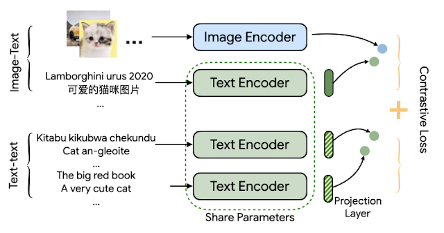
The architecture of MURAL depicts dual encoders with a shared text-encoder between the two tasks trained using a contrastive learning loss.

Multilingual Image-to-Text and Text-to-Image Retrieval
To demonstrate MURAL’s capabilities, we choose the task of cross-modal retrieval (i.e., retrieving relevant images given a text and vice versa) and report the scores on various academic image–text datasets covering well-resourced languages, such as MS-COCO (and its Japanese variant, STAIR), Flickr30K (in English) and Multi30K (extended to German, French, Czech), XTD (test-only set with seven well-resourced languages: Italian, Spanish, Russian, Chinese, Polish, Turkish, and Korean). In addition to well-resourced languages, we also evaluate MURAL on the recently published Wikipedia Image–Text (WIT) dataset, which covers 108 languages, with a broad range of both well-resourced (English, French, Chinese, etc.) and under-resourced (Swahili, Hindi, etc.) languages.

MURAL consistently outperforms prior state-of-the-art models, including M3P, UC2, and ALIGN, in both zero-shot and fine-tuned settings evaluated on well-resourced and under-resourced languages. We see remarkable performance gains for under-resourced languages when compared to the state-of-the-art model, ALIGN.

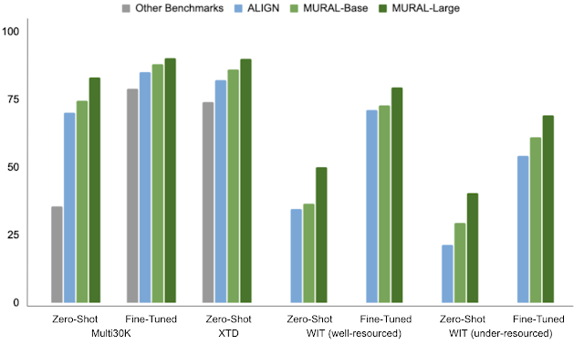
Mean recall on various multilingual image–text retrieval benchmarks. Mean recall is a common metric used to evaluate cross-modal retrieval performance on image–text datasets (higher is better). It measures the Recall@N (i.e., the chance that the ground truth image appears in the first N retrieved images) averaged over six measurements: Image→Text and Text→Image retrieval for N=[1, 5, 10]. Note that XTD scores report Recall@10 for Text→Image retrieval.

Retrieval Analysis
We also analyzed zero-shot retrieved examples on the WIT dataset comparing ALIGN and MURAL for English (en) and Hindi (hi). For under-resourced languages like Hindi, MURAL shows improved retrieval performance compared to ALIGN that reflects a better grasp of the text semantics.

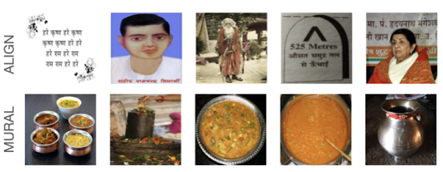
Comparison of the top-5 images retrieved by ALIGN and by MURAL for the Text→Image retrieval task on the WIT dataset for the Hindi text, एक तश्तरी पर बिना मसाले या सब्ज़ी के रखी हुई सादी स्पगॅत्ती”, which translates to the English, “A bowl containing plain noodles without any spices or vegetables”.

Even for Image→Text retrieval in a well-resourced language, like French, MURAL shows better understanding for some words. For example, MURAL returns better results for the query “cadran solaire” (“sundial”, in French) than ALIGN, which doesn’t retrieve any text describing sundials (below).

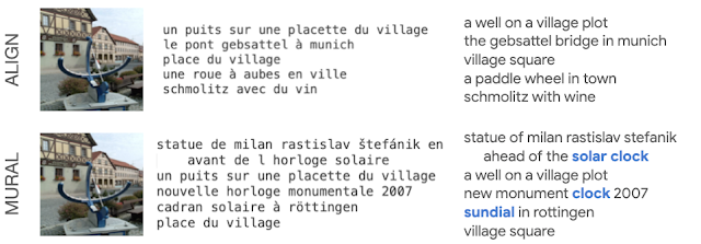
Comparison of the top-5 text results from ALIGN and from MURAL on the Image→Text retrieval task for the same image of a sundial.

Embeddings Visualization
Previously, researchers have shown that visualizing model embeddings can reveal interesting connections among languages — for instance, representations learned by a neural machine translation (NMT) model have been shown to form clusters based on their membership to a language family. We perform a similar visualization for a subset of languages belonging to the Germanic, Romance, Slavic, Uralic, Finnic, Celtic, and Finno-Ugric language families (widely spoken in Europe and Western Asia). We compare MURAL’s text embeddings with LaBSE’s, which is a text-only encoder.

A plot of LabSE’s embeddings shows distinct clusters of languages influenced by language families. For instance, Romance languages (in purple, below) fall into a different region than Slavic languages (in brown, below). This finding is consistent with prior work that investigates intermediate representations learned by a NMT system.

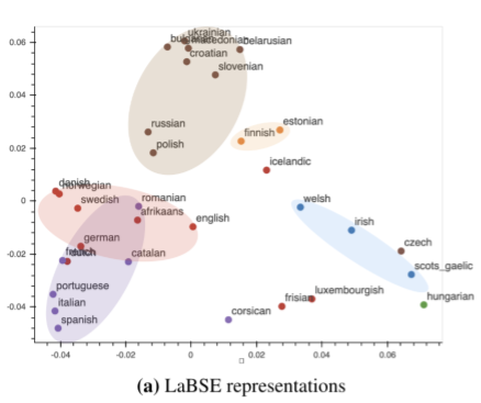
Visualization of text representations of LaBSE for 35 languages. Languages are color coded based on their genealogical association. Representative languages include: Germanic (red) — German, English, Dutch; Uralic (orange) — Finnish, Estonian; Slavic (brown) — Polish, Russian; Romance (purple) — Italian, Portuguese, Spanish; Gaelic (blue) — Welsh, Irish.

In contrast to LaBSE’s visualization, MURAL’s embeddings, which are learned with a multimodal objective, shows some clusters that are in line with areal linguistics (where elements are shared by languages or dialects in a geographic area) and contact linguistics (where languages or dialects interact and influence each other). Notably, in the MURAL embedding space, Romanian (ro) is closer to the Slavic languages like Bulgarian (bg) and Macedonian (mk), which is in line with the Balkan sprachbund, than it is in LaBSE. Another possible language contact brings Finnic languages, Estonian (et) and Finnish (fi), closer to the Slavic languages cluster. The fact that MURAL pivots on images as well as translations appears to add an additional view on language relatedness as learned in deep representations, beyond the language family clustering observed in a text-only setting.

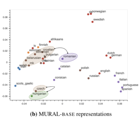
Visualization of text representations of MURAL for 35 languages. Color coding is the same as the figure above.

Final Remarks
Our findings show that training jointly using translation pairs helps overcome the scarcity of image–text pairs for many under-resourced languages and improves cross-modal performance. Additionally, it is interesting to observe hints of areal linguistics and contact linguistics in the text representations learned by using a multimodal model. This warrants more probing into different connections learned implicitly by multimodal models, such as MURAL. Finally, we hope this work promotes further research in the multimodal, multilingual space where models learn representations of and connections between languages (expressed via images and text), beyond well-resourced languages.

Acknowledgements
This research is in collaboration with Mandy Guo, Krishna Srinivasan, Ting Chen, Sneha Kudugunta, Chao Jia, and Jason Baldridge. We thank Zarana Parekh, Orhan Firat, Yuqing Chen, Apu Shah, Anosh Raj, Daphne Luong, and others who provided feedback for the project. We are also grateful for general support from Google Research teams.

Posted by Florian Hartmann, Software Engineer, Google Research

Smart Text Selection, launched in 2017 as part of Android O, is one of Android’s most frequently used features, helping users select, copy, and use text easily and quickly by predicting the desired word or set of words around a user’s tap, and automatically expanding the selection appropriately. Through this feature, selections are automatically expanded, and for selections with defined classification types, e.g., addresses and phone numbers, users are offered an app with which to open the selection, saving users even more time.

Today we describe how we have improved the performance of Smart Text Selection by using federated learning to train the neural network model on user interactions responsibly while preserving user privacy. This work, which is part of Android’s new Private Compute Core secure environment, enabled us to improve the model’s selection accuracy by up to 20% on some types of entities.

Server-Side Proxy Data for Entity Selections
Smart Text Selection, which is the same technology behind Smart Linkify, does not predict arbitrary selections, but focuses on well-defined entities, such as addresses or phone numbers, and tries to predict the selection bounds for those categories. In the absence of multi-word entities, the model is trained to only select a single word in order to minimize the frequency of making multi-word selections in error.

The Smart Text Selection feature was originally trained using proxy data sourced from web pages to which schema.org annotations had been applied. These entities were then embedded in a selection of random text, and the model was trained to select just the entity, without spilling over into the random text surrounding it.

While this approach of training on schema.org-annotations worked, it had several limitations. The data was quite different from text that we expect users see on-device. For example, websites with schema.org annotations typically have entities with more proper formatting than what users might type on their phones. In addition, the text samples in which the entities were embedded for training were random and did not reflect realistic context on-device.

On-Device Feedback Signal for Federated Learning
With this new launch, the model no longer uses proxy data for span prediction, but is instead trained on-device on real interactions using federated learning. This is a training approach for machine learning models in which a central server coordinates model training that is split among many devices, while the raw data used stays on the local device. A standard federated learning training process works as follows: The server starts by initializing the model. Then, an iterative process begins in which (a) devices get sampled, (b) selected devices improve the model using their local data, and (c) then send back only the improved model, not the data used for training. The server then averages the updates it received to create the model that is sent out in the next iteration.

For Smart Text Selection, each time a user taps to select text and corrects the model’s suggestion, Android gets precise feedback for what selection span the model should have predicted. In order to preserve user privacy, the selections are temporarily kept on the device, without being visible server-side, and are then used to improve the model by applying federated learning techniques. This technique has the advantage of training the model on the same kind of data that it sees during inference.

Federated Learning & Privacy
One of the advantages of the federated learning approach is that it enables user privacy, because raw data is not exposed to a server. Instead, the server only receives updated model weights. Still, to protect against various threats, we explored ways to protect the on-device data, securely aggregate gradients, and reduce the risk of model memorization.

The on-device code for training Federated Smart Text Selection models is part of Android’s Private Compute Core secure environment, which makes it particularly well situated to securely handle user data. This is because the training environment in Private Compute Core is isolated from the network and data egress is only allowed when federated and other privacy-preserving techniques are applied. In addition to network isolation, data in Private Compute Core is protected by policies that restrict how it can be used, thus protecting from malicious code that may have found its way onto the device.

To aggregate model updates produced by the on-device training code, we use Secure Aggregation, a cryptographic protocol that allows servers to compute the mean update for federated learning model training without reading the updates provided by individual devices. In addition to being individually protected by Secure Aggregation, the updates are also protected by transport encryption, creating two layers of defense against attackers on the network.

Finally, we looked into model memorization. In principle, it is possible for characteristics of the training data to be encoded in the updates sent to the server, survive the aggregation process, and end up being memorized by the global model. This could make it possible for an attacker to attempt to reconstruct the training data from the model. We used methods from Secret Sharer, an analysis technique that quantifies to what degree a model unintentionally memorizes its training data, to empirically verify that the model was not memorizing sensitive information. Further, we employed data masking techniques to prevent certain kinds of sensitive data from ever being seen by the model

In combination, these techniques help ensure that Federated Smart Text Selection is trained in a way that preserves user privacy.

Achieving Superior Model Quality
Initial attempts to train the model using federated learning were unsuccessful. The loss did not converge and predictions were essentially random. Debugging the training process was difficult, because the training data was on-device and not centrally collected, and so, it could not be examined or verified. In fact, in such a case, it’s not even possible to determine if the data looks as expected, which is often the first step in debugging machine learning pipelines.

To overcome this challenge, we carefully designed high-level metrics that gave us an understanding of how the model behaved during training. Such metrics included the number of training examples, selection accuracy, and recall and precision metrics for each entity type. These metrics are collected during federated training via federated analytics, a similar process as the collection of the model weights. Through these metrics and many analyses, we were able to better understand which aspects of the system worked well and where bugs could exist.

After fixing these bugs and making additional improvements, such as implementing on-device filters for data, using better federated optimization methods and applying more robust gradient aggregators, the model trained nicely.

Results
Using this new federated approach, we were able to significantly improve Smart Text Selection models, with the degree depending on the language being used. Typical improvements ranged between 5% and 7% for multi-word selection accuracy, with no drop in single-word performance. The accuracy of correctly selecting addresses (the most complex type of entity supported) increased by between 8% and 20%, again, depending on the language being used. These improvements lead to millions of additional selections being automatically expanded for users every day.

Internationalization
An additional advantage of this federated learning approach for Smart Text Selection is its ability to scale to additional languages. Server-side training required manual tweaking of the proxy data for each language in order to make it more similar to on-device data. While this only works to some degree, it takes a tremendous amount of effort for each additional language.

The federated learning pipeline, however, trains on user interactions, without the need for such manual adjustments. Once the model achieved good results for English, we applied the same pipeline to Japanese and saw even greater improvements, without needing to tune the system specifically for Japanese selections.

We hope that this new federated approach lets us scale Smart Text Selection to many more languages. Ideally this will also work without manual tuning of the system, making it possible to support even low-resource languages.

Conclusion
We developed a federated way of learning to predict text selections based on user interactions, resulting in much improved Smart Text Selection models deployed to Android users. This approach required the use of federated learning, since it works without collecting user data on the server. Additionally, we used many state-of-the-art privacy approaches, such as Android’s new Private Compute Core, Secure Aggregation and the Secret Sharer method. The results show that privacy does not have to be a limiting factor when training models. Instead, we managed to obtain a significantly better model, while ensuring that users’ data stays private.

Acknowledgements
Many people contributed to this work. We would like to thank Lukas Zilka, Asela Gunawardana, Silvano Bonacina, Seth Welna, Tony Mak, Chang Li, Abodunrinwa Toki, Sergey Volnov, Matt Sharifi, Abhanshu Sharma, Eugenio Marchiori, Jacek Jurewicz, Nicholas Carlini, Jordan McClead, Sophia Kovaleva, Evelyn Kao, Tom Hume, Alex Ingerman, Brendan McMahan, Fei Zheng, Zachary Charles, Sean Augenstein, Zachary Garrett, Stefan Dierauf, David Petrou, Vishwath Mohan, Hunter King, Emily Glanz, Hubert Eichner, Krzysztof Ostrowski, Jakub Konecny, Shanshan Wu, Janel Thamkul, Elizabeth Kemp, and everyone else involved in the project.

Posted by Pete Florence, Research Scientist and Corey Lynch, Research Engineer, Robotics at Google

Despite considerable progress in robot learning over the past several years, some policies for robotic agents can still struggle to decisively choose actions when trying to imitate precise or complex behaviors. Consider a task in which a robot tries to slide a block across a table to precisely position it into a slot. There are many possible ways to solve this task, each requiring precise movements and corrections. The robot must commit to just one of these options, but must also be capable of changing plans each time the block ends up sliding farther than expected. Although one might expect such a task to be easy, that is often not the case for modern learning-based robots, which often learn behavior that expert observers describe as indecisive or imprecise.

Example of a baseline explicit behavior cloning model struggling on a task where the robot needs to slide a block across a table and then precisely insert it into a fixture.

To encourage robots to be more decisive, researchers often utilize a discretized action space, which forces the robot to choose option A or option B, without oscillating between options. For example, discretization was a key element of our recent Transporter Networks architecture, and is also inherent in many notable achievements by game-playing agents, such as AlphaGo, AlphaStar, and OpenAI’s Dota bot. But discretization brings its own limitations — for robots that operate in the spatially continuous real world, there are at least two downsides to discretization: (i) it limits precision, and (ii) it triggers the curse of dimensionality, since considering discretizations along many different dimensions can dramatically increase memory and compute requirements. Related to this, in 3D computer vision much recent progress has been powered by continuous, rather than discretized, representations.

With the goal of learning decisive policies without the drawbacks of discretization, today we announce our open source implementation of Implicit Behavioral Cloning (Implicit BC), which is a new, simple approach to imitation learning and was presented last week at CoRL 2021. We found that Implicit BC achieves strong results on both simulated benchmark tasks and on real-world robotic tasks that demand precise and decisive behavior. This includes achieving state-of-the-art (SOTA) results on human-expert tasks from our team’s recent benchmark for offline reinforcement learning, D4RL. On six out of seven of these tasks, Implicit BC outperforms the best previous method for offline RL, Conservative Q Learning. Interestingly, Implicit BC achieves these results without requiring any reward information, i.e., it can use relatively simple supervised learning rather than more-complex reinforcement learning.

Implicit Behavioral Cloning
Our approach is a type of behavior cloning, which is arguably the simplest way for robots to learn new skills from demonstrations. In behavior cloning, an agent learns how to mimic an expert’s behavior using standard supervised learning. Traditionally, behavior cloning involves training an explicit neural network (shown below, left), which takes in observations and outputs expert actions.

The key idea behind Implicit BC is to instead train a neural network to take in both observations and actions, and output a single number that is low for expert actions and high for non-expert actions (below, right), turning behavioral cloning into an energy-based modeling problem. After training, the Implicit BC policy generates actions by finding the action input that has the lowest score for a given observation.

Depiction of the difference between explicit (left) and implicit (right) policies. In the implicit policy, the “argmin” means the action that, when paired with a particular observation, minimizes the value of the energy function.

To train Implicit BC models, we use an InfoNCE loss, which trains the network to output low energy for expert actions in the dataset, and high energy for all others (see below). It is interesting to note that this idea of using models that take in both observations and actions is common in reinforcement learning, but not so in supervised policy learning.

Animation of how implicit models can fit discontinuities — in this case, training an implicit model to fit a step (Heaviside) function. Left: 2D plot fitting the black (X) training points — the colors represent the values of the energies (blue is low, brown is high). Middle: 3D plot of the energy model during training. Right: Training loss curve.

Once trained, we find that implicit models are particularly good at precisely modeling discontinuities (above) on which prior explicit models struggle (as in the first figure of this post), resulting in policies that are newly capable of switching decisively between different behaviors.

But why do conventional explicit models struggle? Modern neural networks almost always use continuous activation functions — for example, Tensorflow, Jax, and PyTorch all only ship with continuous activation functions. In attempting to fit discontinuous data, explicit networks built with these activation functions cannot represent discontinuities, so must draw continuous curves between data points. A key aspect of implicit models is that they gain the ability to represent sharp discontinuities, even though the network itself is composed only of continuous layers.

We also establish theoretical foundations for this aspect, specifically a notion of universal approximation. This proves the class of functions that implicit neural networks can represent, which can help justify and guide future research.

Examples of fitting discontinuous functions, for implicit models (top) compared to explicit models (bottom). The red highlighted insets show that implicit models represent discontinuities (a) and (b) while the explicit models must draw continuous lines (c) and (d) in between the discontinuities.

One challenge faced by our initial attempts at this approach was “high action dimensionality”, which means that a robot must decide how to coordinate many motors all at the same time. To scale to high action dimensionality, we use either autoregressive models or Langevin dynamics.

Highlights
In our experiments, we found Implicit BC does particularly well in the real world, including an order of magnitude (10x) better on the 1mm-precision slide-then-insert task compared to a baseline explicit BC model. On this task the implicit model does several consecutive precise adjustments (below) before sliding the block into place. This task demands multiple elements of decisiveness: there are many different possible solutions due to the symmetry of the block and the arbitrary ordering of push maneuvers, and the robot needs to discontinuously decide when the block has been pushed far “enough” before switching to slide it in a different direction. This is in contrast to the indecisiveness that is often associated with continuous-controlled robots.

Example task of sliding a block across a table and precisely inserting it into a slot. These are autonomous behaviors of our Implicit BC policies, using only images (from the shown camera) as input.

A diverse set of different strategies for accomplishing this task. These are autonomous behaviors from our Implicit BC policies, using only images as input.

In another challenging task, the robot needs to sort blocks by color, which presents a large number of possible solutions due to the arbitrary ordering of sorting. On this task the explicit models are customarily indecisive, while implicit models perform considerably better.

Comparison of implicit (left) and explicit (right) BC models on a challenging continuous multi-item sorting task. (4x speed)

In our testing, implicit BC models can also exhibit robust reactive behavior, even when we try to interfere with the robot, despite the model never seeing human hands.

Robust behavior of the implicit BC model despite interfering with the robot.

Overall, we find that Implicit BC policies can achieve strong results compared to state of the art offline reinforcement learning methods across several different task domains. These results include tasks that, challengingly, have either a low number of demonstrations (as few as 19), high observation dimensionality with image-based observations, and/or high action dimensionality up to 30 — which is a large number of actuators to have on a robot.

Policy learning results of Implicit BC compared to baselines across several domains.

Conclusion
Despite its limitations, behavioral cloning with supervised learning remains one of the simplest ways for robots to learn from examples of human behaviors. As we showed here, replacing explicit policies with implicit policies when doing behavioral cloning allows robots to overcome the “struggle of decisiveness”, enabling them to imitate much more complex and precise behaviors. While the focus of our results here was on robot learning, the ability of implicit functions to model sharp discontinuities and multimodal labels may have broader interest in other application domains of machine learning as well.

Acknowledgements
Pete and Corey summarized research performed together with other co-authors: Andy Zeng, Oscar Ramirez, Ayzaan Wahid, Laura Downs, Adrian Wong, Johnny Lee, Igor Mordatch, and Jonathan Tompson. The authors would also like to thank Vikas Sindwhani for project direction advice; Steve Xu, Robert Baruch, Arnab Bose for robot software infrastructure; Jake Varley, Alexa Greenberg for ML infrastructure; and Kamyar Ghasemipour, Jon Barron, Eric Jang, Stephen Tu, Sumeet Singh, Jean-Jacques Slotine, Anirudha Majumdar, Vincent Vanhoucke for helpful feedback and discussions.

Posted by David Ha, Staff Research Scientist and Yujin Tang, Research Software Engineer, Google Research, Tokyo

“The brain is able to use information coming from the skin as if it were coming from the eyes. We don’t see with the eyes or hear with the ears, these are just the receptors, seeing and hearing in fact goes on in the brain.”

– Paul Bach-y-Rita¹

People have the amazing ability to use one sensory modality (e.g., touch) to supply environmental information normally gathered by another sense (e.g., vision). This adaptive ability, called sensory substitution, is a phenomenon well-known to neuroscience. While difficult adaptations — such as adjusting to seeing things upside-down, learning to ride a “backwards” bicycle, or learning to “see” by interpreting visual information emitted from a grid of electrodes placed on one’s tongue — require anywhere from weeks, months or even years to attain mastery, people are able to eventually adjust to sensory substitutions.

<!–

–>

Examples of Sensory Substitution. Left: Tongue Display Unit (Maris and Bach-y-Rita, 2001; Image: Kaczmarek, 2011). Right: “Upside down goggles” initially conceived by Erismann and Kohler in 1931. (Image Wikipedia).

In contrast, most neural networks are not able to adapt to sensory substitutions at all. For instance, most reinforcement learning (RL) agents require their inputs to be in a pre-specified format, or else they will fail. They expect fixed-size inputs and assume that each element of the input carries a precise meaning, such as the pixel intensity at a specified location, or state information, like position or velocity. In popular RL benchmark tasks (e.g., Ant or Cart-pole), an agent trained using current RL algorithms will fail if its sensory inputs are changed or if the agent is fed additional noisy inputs that are unrelated to the task at hand.

In “The Sensory Neuron as a Transformer: Permutation-Invariant Neural Networks for Reinforcement Learning”, a spotlight paper at NeurIPS 2021, we explore permutation invariant neural network agents, which require each of their sensory neurons (receptors that receive sensory inputs from the environment) to figure out the meaning and context of its input signal, rather than explicitly assuming a fixed meaning. Our experiments show that such agents are robust to observations that contain additional redundant or noisy information, and to observations that are corrupt and incomplete.

Permutation invariant reinforcement learning agents adapting to sensory substitutions. Left: The ordering of the ant’s 28 observations are randomly shuffled every 200 time-steps. Unlike the standard policy, our policy is not affected by the suddenly permuted inputs. Right: Cart-pole agent given many redundant noisy inputs (Interactive web-demo).

In addition to adapting to sensory substitutions in state-observation environments (like the ant and cart-pole examples), we show that these agents can also adapt to sensory substitutions in complex visual-observation environments (such as a CarRacing game that uses only pixel observations) and can perform when the stream of input images is constantly being reshuffled:

We partition the visual input from CarRacing into a 2D grid of small patches, and shuffled their ordering. Without any additional training, our agent still performs even when the original training background (left) is replaced with new images (right).

Method
Our approach takes observations from the environment at each time-step and feeds each element of the observation into distinct, but identical neural networks (called “sensory neurons”), each with no fixed relationship with one another. Each sensory neuron integrates over time information from only their particular sensory input channel. Because each sensory neuron receives only a small part of the full picture, they need to self-organize through communication in order for a global coherent behavior to emerge.

Illustration of observation segmentation.We segment each input into elements, which are then fed to independent sensory neurons. For non-vision tasks where the inputs are usually 1D vectors, each element is a scalar. For vision tasks, we crop each input image into non-overlapping patches.

We encourage neurons to communicate with each other by training them to broadcast messages. While receiving information locally, each individual sensory neuron also continually broadcasts an output message at each time-step. These messages are consolidated and combined into an output vector, called the global latent code, using an attention mechanism similar to that applied in the Transformer architecture. A policy network then uses the global latent code to produce the action that the agent will use to interact with the environment. This action is also fed back into each sensory neuron in the next time-step, closing the communication loop.

Overview of the permutation-invariant RL method. We first feed each individual observation (ot) into a particular sensory neuron (along with the agent’s previous action, at-1). Each neuron then produces and broadcasts a message independently, and an attention mechanism summarizes them into a global latent code (mt) that is given to the agent’s downstream policy network (𝜋) to produce the agent’s action at.

Why is this system permutation invariant? Each sensory neuron is an identical neural network that is not confined to only process information from one particular sensory input. In fact, in our setup, the inputs to each sensory neuron are not defined. Instead, each neuron must figure out the meaning of its input signal by paying attention to the inputs received by the other sensory neurons, rather than explicitly assuming a fixed meaning. This encourages the agent to process the entire input as an unordered set, making the system to be permutation invariant to its input. Furthermore, in principle, the agent can use as many sensory neurons as required, thus enabling it to process observations of arbitrary length. Both of these properties will help the agent adapt to sensory substitutions.

Results
We demonstrate the robustness and flexibility of this approach in simpler, state-observation environments, where the observations the agent receives as inputs are low-dimensional vectors holding information about the agent’s states, such as the position or velocity of its components. The agent in the popular Ant locomotion task has a total of 28 inputs with information that includes positions and velocities. We shuffle the order of the input vector several times during a trial and show that the agent is rapidly able to adapt and is still able to walk forward.

In cart-pole, the agent’s goal is to swing up a cart-pole mounted at the center of the cart and balance it upright. Normally the agent sees only five inputs, but we modify the cartpole environment to provide 15 shuffled input signals, 10 of which are pure noise, and the remainder of which are the actual observations from the environment. The agent is still able to perform the task, demonstrating the system’s capacity to work with a large number of inputs and attend only to channels it deems useful. Such flexibility may find useful applications for processing a large unspecified number of signals, most of which are noise, from ill-defined systems.

We also apply this approach to high-dimensional vision-based environments where the observation is a stream of pixel images. Here, we investigate screen-shuffled versions of vision-based RL environments, where each observation frame is divided into a grid of patches, and like a puzzle, the agent must process the patches in a shuffled order to determine a course of action to take. To demonstrate our approach on vision-based tasks, we created a shuffled version of Atari Pong.

Shuffled Pong results. Left: Pong agent trained to play using only 30% of the patches matches performance of Atari opponent. Right: Without extra training, when we give the agent more puzzle pieces, its performance increases.

Here the agent’s input is a variable-length list of patches, so unlike typical RL agents, the agent only gets to “see” a subset of patches from the screen. In the puzzle pong experiment, we pass to the agent a random sample of patches across the screen, which are then fixed through the remainder of the game. We find that we can discard 70% of the patches (at these fixed-random locations) and still train the agent to perform well against the built-in Atari opponent. Interestingly, if we then reveal additional information to the agent (e.g., allowing it access to more image patches), its performance increases, even without additional training. When the agent receives all the patches, in shuffled order, it wins 100% of the time, achieving the same result with agents that are trained while seeing the entire screen.

We find that imposing additional difficulty during training by using unordered observations has additional benefits, such as improving generalization to unseen variations of the task, like when the background of the CarRacing training environment is replaced with a novel image.

Shuffled CarRacing results. The agent has learned to focus its attention (indicated by the highlighted patches) on the road boundaries. Left: Training environment. Right: Test environment with new background.

Conclusion
The permutation invariant neural network agents presented here can handle ill-defined, varying observation spaces. Our agents are robust to observations that contain redundant or noisy information, or observations that are corrupt and incomplete. We believe that permutation invariant systems open up numerous possibilities in reinforcement learning.

If you’re interested to learn more about this work, we invite readers to read our interactive article (pdf version) or watch our video. We also released code to reproduce our experiments.

---

¹Quoted in Livewired, by David Eagleman.  ^↩

For a while, it may have seemed that Keras for R was in some undecidable state, like Schrödinger’s cat before inspection. It is high time to correct that impression. Keras for R is back, with two recent releases adding powerful capabilities that considerably lighten previously tedious tasks. This post provides a high-level overview. Future posts will go into more detail on some of the most helpful new features, as well as dive into the powerful low-level enhancements that make the former possible.

Posted by Sian Gooding, Intern, Google Research

Illiteracy affects at least 773 million people globally, both young and old. For these individuals, reading information from unfamiliar sources or on unfamiliar topics can be extremely difficult. Unfortunately, these inequalities have been further magnified by the global pandemic as a result of unequal access to education in reading and writing. In fact, UNESCO reports that over 100 million children are falling behind the minimum proficiency level in reading due to COVID-related school closures.

With increasing world-wide access to technology, reading on a device, such as a tablet or phone, has largely taken the place of traditional formats. This provides a unique opportunity to observe reading interactions, e.g., how a reader scrolls through a text, which can inform our understanding of what can make text difficult to read. This understanding is crucial when designing educational applications for low-proficiency readers and language learners, because it can be used to match learners with appropriately leveled texts as well as to support readers in understanding texts beyond their reading level.

In “Predicting Text Readability from Scrolling Interactions”, presented at CoNLL 2021, we show that data from on-device reading interactions can be used to predict how readable a text is. This novel approach provides insights into subjective readability — whether an individual reader has found a text accessible — and demonstrates that existing readability models can be improved by including feedback from scroll-based reading interactions. In order to encourage research in this area and to help enable more personalized tools for language learning and text simplification, we are releasing the dataset of reading interactions generated from our scrolling behavior–based readability assessment of English-language texts.

Understanding Text Difficulty
There are multiple aspects of a text that impact how difficult it is to read, including the vocabulary level, the syntactic structure, and overall coherence. Traditional machine learning approaches to measure readability have exclusively relied on such linguistic features. However, using these features alone does not work well for online content, because such content often contains abbreviations, emojis, broken text, and short passages, which detrimentally impact the performance of readability models.

To address this, we investigated whether aggregate data about the reading interactions of a group can be used to predict how difficult a text is, as well as how reading interactions may differ based on a readers’ understanding. When reading on a device, readers typically interact with text by scrolling in a vertical fashion, which we hypothesize can be used as a coarse proxy for reading comprehension. With this in mind, we recruited 518 paid participants and asked them to read English-language texts of different difficulty levels. We recorded the reading interactions by measuring different features of the participants’ scrolling behavior, such as the speed, acceleration and number of times areas of text were revisited. We then used this information to produce a set of features for a readability classifier.

Predicting Text Difficulty from Scrolling Behavior
We investigated which types of scrolling behaviors were most impacted by text difficulty and tested the significance using linear mixed effect models. In our set up, we have repeated measures, as multiple participants read the same texts and each participant reads more than one text. Using linear mixed-effect models gives us a higher confidence that the differences in interactions we are observing are because of the text difficulty, and not other random effects.

Our results showed that multiple reading behaviors differed significantly based on the text level, for example, the average, maximum and minimum acceleration of scrolling. We found the most significant features to be the total read time and the maximum reading speeds.

We then used these features as inputs to a machine learning algorithm. We designed and trained a support vector machine (i.e., a binary classifier) to predict whether a text is either advanced or elementary based only on scrolling behaviors as individuals interacted with it. The dataset on which the model was trained contains 60 articles, each of which were read by an average of 17 participants. From these interactions we produced aggregate features by taking the mean of the significant measures across participants.

 

We measured the accuracy of the approach using a metric called f-score, which measures how accurate the model is at classifying a text as either “easy” or “difficult” (where 1.0 reflects perfect classification accuracy). We are able to achieve an f-score of 0.77 on this task, using interaction features alone. This is the first work to show that it is possible to predict the readability of a text using only interaction features.

Improving Readability Models
In order to demonstrate the value of applying readability measures from scrolling behaviors to existing readability models, we integrated scroll-based features into the state-of-the-art automated readability assessment tool, which was released as part of the OneStopEnglish corpus. We found that the addition of interaction features improves the f-score of this model from 0.84 to 0.88. In addition, we were able to significantly outperform this system by using interaction information with simple vocabulary features, such as the number of words in the text, achieving an impressive f-score of 0.96.

In our study, we recorded comprehension scores to evaluate the understanding and readability of text for individuals. Participants were asked three questions per article to assess the reader’s understanding of what they had read. The interaction features of an individual’s scrolling behavior was represented as a high dimensional vector. To explore this data, we visualized the reading interaction features for each participant using t-distributed stochastic neighbor embeddings, which is a statistical method for visualizing high-dimensional data. The results revealed clusters in the comprehension score based on how well individuals understood the text. This shows that there is implicit information in reading interactions about the likelihood that an individual has understood a given text. We refer to this phenomenon as subjective readability. This information can be very useful for educational applications or for simplifying online content.

Plot showing t-SNE projection of scroll interactions in 2-dimensions. The color of each data point corresponds to the comprehension score. Clusters of comprehension scores indicate that there are correlations between reading behaviors and comprehension.

Finally, we investigated the extent to which reading interactions vary across audiences. We compared the average scrolling speed across different reader groups, covering reading proficiency and the reader’s first language. We found that the speed distribution varies depending on the proficiency and first language of the audience. This supports the case that first language and proficiency alter the reading behaviors of audiences, which allows us to contextualize the reading behavior of groups and better understand which areas of text may be harder for them to read.

Histogram showing the average speeds of scrolling (in vertical pixels per millisecond) across readers of different proficiency levels (beginner, intermediate and advanced), with lines showing the smoothed trend for each group. A higher average scroll speed indicates faster reading times. For example, a more challenging text that corresponds to slower scroll speeds by advanced readers is associated with higher scroll speeds by beginners because they engage with the text only superficially.

Histogram showing the average speeds of scrolling (in vertical pixels per millisecond) across audiences by first language of the readers, Tamil or English, with lines showing the smoothed trend for each group. A higher average scroll speed indicates faster reading times. Dark blue bars are where the histograms overlap.

Conclusion
This work is the first to show that reading interactions, such as scrolling behavior, can be used to predict the readability of text, which can yield numerous benefits. Such measures are language agnostic, unobtrusive, and robust to noisy text. Implicit user feedback allows insight into readability at an individual level, thereby allowing for a more inclusive and personalisable assessment of text difficulty. Furthermore, being able to judge the subjective readability of text benefits language learning and educational apps. We conducted a 518 participant study to investigate the impact of text readability on reading interactions and are releasing a novel dataset of the associated reading interactions. We confirm that there are statistically significant differences in the way that readers interact with advanced and elementary texts, and that the comprehension scores of individuals correlate with specific measures of scrolling interaction. For more information our conference presentation is available to view.

Acknowledgements
We thank our collaborators Yevgeni Berzak, Tony Mak and Matt Sharifi, as well as Dmitry Lagun and Blaise Aguera y Arcas for their helpful feedback on the paper.

Posted by Rishabh Agarwal, Research Scientist and Pablo Samuel Castro, Staff Software Engineer, Google Research, Brain Team

Reinforcement learning (RL) is an area of machine learning that focuses on learning from experiences to solve decision making tasks. While the field of RL has made great progress, resulting in impressive empirical results on complex tasks, such as playing video games, flying stratospheric balloons and designing hardware chips, it is becoming increasingly apparent that the current standards for empirical evaluation might give a false sense of fast scientific progress while slowing it down.

To that end, in “Deep RL at the Edge of the Statistical Precipice”, accepted as an oral presentation at NeurIPS 2021, we discuss how statistical uncertainty of results needs to be considered, especially when using only a few training runs, in order for evaluation in deep RL to be reliable. Specifically, the predominant practice of reporting point estimates ignores this uncertainty and hinders reproducibility of results. Related to this, tables with per-task scores, as are commonly reported, can be overwhelming beyond a few tasks and often omit standard deviations. Furthermore, simple performance metrics like the mean can be dominated by a few outlier tasks, while the median score would remain unaffected even if up to half of the tasks had performance scores of zero. Thus, to increase the field’s confidence in reported results with a handful of runs, we propose various statistical tools, including stratified bootstrap confidence intervals, performance profiles, and better metrics, such as interquartile mean and probability of improvement. To help researchers incorporate these tools, we also release an easy-to-use Python library RLiable with a quickstart colab.

Statistical Uncertainty in RL Evaluation
Empirical research in RL relies on evaluating performance on a diverse suite of tasks, such as Atari 2600 video games, to assess progress. Published results on deep RL benchmarks typically compare point estimates of the mean and median scores aggregated across tasks. These scores are typically relative to some defined baseline and optimal performance (e.g., random agent and “average” human performance on Atari games, respectively) so as to make scores comparable across different tasks.

In most RL experiments, there is randomness in the scores obtained from different training runs, so reporting only point estimates does not reveal whether similar results would be obtained with new independent runs. A small number of training runs, coupled with the high variability in performance of deep RL algorithms, often leads to large statistical uncertainty in such point estimates.

The distribution of median human normalized scores on the Atari 100k benchmark, which contains 26 games, for five recently published algorithms, DER, OTR, CURL, two variants of DrQ, and SPR. The reported point estimates of median scores based on a few runs in publications, as shown by dashed lines, do not provide information about the variability in median scores and typically overestimate (e.g., CURL, SPR, DrQ) or underestimate (e.g., DER) the expected median, which can result in erroneous conclusions.

As benchmarks become increasingly more complex, evaluating more than a few runs will be increasingly demanding due to the increased compute and data needed to solve such tasks. For example, five runs on 50 Atari games for 200 million frames takes 1000+ GPU days. Thus, evaluating more runs is not a feasible solution for reducing statistical uncertainty on computationally demanding benchmarks. While prior work has recommended statistical significance tests as a solution, such tests are dichotomous in nature (either “significant” or “not significant”), so they often lack the granularity needed to yield meaningful insights and are widely misinterpreted.

Number of runs in RL papers over the years. Beginning with the Arcade Learning Environment (ALE), the shift toward computationally-demanding benchmarks has led to the practice of evaluating only a handful of runs per task, increasing the statistical uncertainty in point estimates.

Tools for Reliable Evaluation
Any aggregate metric based on a finite number of runs is a random variable, so to take this into account, we advocate for reporting stratified bootstrap confidence intervals (CIs), which predict the likely values of aggregate metrics if the same experiment were repeated with different runs. These CIs allow us to understand the statistical uncertainty and reproducibility of results. Such CIs use the scores on combined runs across tasks. For example, evaluating 3 runs each on Atari 100k, which contains 26 tasks, results in 78 sample scores for uncertainty estimation.

In each task, colored balls denote scores on different runs. To compute statified bootstrap CIs using the percentile method, bootstrap samples are created by randomly sampling scores with replacement proportionately from each task. Then, the distribution of aggregate scores on these samples is the bootstrapping distribution, whose spread around the center gives us the confidence interval.

Most deep RL algorithms often perform better on some tasks and training runs, but aggregate performance metrics can conceal this variability, as shown below.

Data with varied appearance but identical aggregate statistics. Source: Same Stats, Different Graphs.

Instead, we recommend performance profiles, which are typically used for comparing solve times of optimization software. These profiles plot the score distribution across all runs and tasks with uncertainty estimates using stratified bootstrap confidence bands. These plots show the total runs across all tasks that obtain a score above a threshold (𝝉) as a function of the threshold.

Performance profiles correspond to the empirical tail distribution of scores on runs combined across all tasks. Shaded regions show 95% stratified bootstrap confidence bands.

Such profiles allow for qualitative comparisons at a glance. For example, the curve for one algorithm above another means that one algorithm is better than the other. We can also read any score percentile, e.g., the profiles intersect y = 0.5 (dotted line above) at the median score. Furthermore, the area under the profile corresponds to the mean score.

While performance profiles are useful for qualitative comparisons, algorithms rarely outperform other algorithms on all tasks and thus their profiles often intersect, so finer quantitative comparisons require aggregate performance metrics. However, existing metrics have limitations: (1) a single high performing task may dominate the task mean score, while (2) the task median is unaffected by zero scores on nearly half of the tasks and requires a large number of training runs for small statistical uncertainty. To address the above limitations, we recommend two alternatives based on robust statistics: the interquartile mean (IQM) and the optimality gap, both of which can be read as areas under the performance profile, below.

IQM (red) corresponds to the area under the performance profile, shown in blue, between the 25 and 75 percentile scores on the x-axis. Optimality gap (yellow) corresponds to the area between the profile and horizontal line at y = 1 (human performance), for scores less than 1.

As an alternative to median and mean, IQM corresponds to the mean score of the middle 50% of the runs combined across all tasks. It is more robust to outliers than mean, a better indicator of overall performance than median, and results in smaller CIs, and so, requires fewer runs to claim improvements. Another alternative to mean, optimality gap measures how far an algorithm is from optimal performance.

IQM discards the lowest 25% and highest 25% of the combined scores (colored balls) and computes the mean of the remaining 50% scores.

For directly comparing two algorithms, another metric to consider is the average probability of improvement, which describes how likely an improvement over baseline is, regardless of its size. This metric is computed using the Mann-Whitney U-statistic, averaged across tasks.

Re-evaluating Evaluation
Using the above tools for evaluation, we revisit performance evaluations of existing algorithms on widely used RL benchmarks, revealing inconsistencies in prior evaluation. For example, in the Arcade Learning Environment (ALE), a widely recognized RL benchmark, the performance ranking of algorithms changes depending on the choice of aggregate metric. Since performance profiles capture the full picture, they often illustrate why such inconsistencies exist.

Median (left) and IQM (right) human normalized scores on the ALE as a function of the number of environment frames seen during training. IQM results in significantly smaller CIs than median scores.

On DM Control, a popular continuous control benchmark, there are large overlaps in 95% CIs of mean normalized scores for most algorithms.

DM Control Suite results, averaged across six tasks, on the 100k and 500k step benchmark. Since scores are normalized using maximum performance, mean scores correspond to one minus the optimality gap. The ordering of the algorithms is based on their claimed relative performance — all algorithms except Dreamer claimed improvement over at least one algorithm placed below them. Shaded regions show 95% CIs.

Finally, on Procgen, a benchmark for evaluating generalization in RL, the average probability of improvement shows that some claimed improvements are only 50-70% likely, suggesting that some reported improvements could be spurious.

Each row shows the probability that the algorithm X on the left outperforms algorithm Y on the right, given that X was claimed to be better than Y. Shaded region denotes 95% stratified bootstrap CIs.

Conclusion
Our findings on widely-used deep RL benchmarks show that statistical issues can have a large influence on previously reported results. In this work, we take a fresh look at evaluation to improve the interpretation of reported results and standardize experimental reporting. We’d like to emphasize the importance of published papers providing results for all runs to allow for future statistical analyses. To build confidence in your results, please check out our open-source library RLiable and the quickstart colab.

Acknowledgments
This work was done in collaboration with Max Schwarzer, Aaron Courville and Marc G. Bellemare. We’d like to thank Tom Small for an animated figure used in this post. We are also grateful for feedback by several members of the Google Research, Brain Team and DeepMind.

Posted by Nal Kalchbrenner and Lasse Espeholt, Google Research

Deep learning has successfully been applied to a wide range of important challenges, such as cancer prevention and increasing accessibility. The application of deep learning models to weather forecasts can be relevant to people on a day-to-day basis, from helping people plan their day to managing food production, transportation systems, or the energy grid. Weather forecasts typically rely on traditional physics-based techniques powered by the world’s largest supercomputers. Such methods are constrained by high computational requirements and are sensitive to approximations of the physical laws on which they are based.

Deep learning offers a new approach to computing forecasts. Rather than incorporating explicit physical laws, deep learning models learn to predict weather patterns directly from observed data and are able to compute predictions faster than physics-based techniques. These approaches also have the potential to increase the frequency, scope, and accuracy of the predicted forecasts.

Illustration of the computation through MetNet-2. As the computation progresses, the network processes an ever larger context from the input and makes a probabilistic forecast of the likely future weather conditions.

Within weather forecasting, deep learning techniques have shown particular promise for nowcasting — i.e., predicting weather up to 2-6 hours ahead. Previous work has focused on using direct neural network models for weather data, extending neural forecasts from 0 to 8 hours with the MetNet architecture, generating continuations of radar data for up to 90 minutes ahead, and interpreting the weather information learned by these neural networks. Still, there is an opportunity for deep learning to extend improvements to longer-range forecasts.

To that end, in “Skillful Twelve Hour Precipitation Forecasts Using Large Context Neural Networks”, we push the forecasting boundaries of our neural precipitation model to 12 hour predictions while keeping a spatial resolution of 1 km and a time resolution of 2 minutes. By quadrupling the input context, adopting a richer weather input state, and extending the architecture to capture longer-range spatial dependencies, MetNet-2 substantially improves on the performance of its predecessor, MetNet. Compared to physics-based models, MetNet-2 outperforms the state-of-the-art HREF ensemble model for weather forecasts up to 12 hours ahead.

MetNet-2 Features and Architecture
Neural weather models like MetNet-2 map observations of the Earth to the probability of weather events, such as the likelihood of rain over a city in the afternoon, of wind gusts reaching 20 knots, or of a sunny day ahead. End-to-end deep learning has the potential to both streamline and increase quality by directly connecting a system’s inputs and outputs. With this in mind, MetNet-2 aims to minimize both the complexity and the total number of steps involved in creating a forecast.

The inputs to MetNet-2 include the radar and satellite images also used in MetNet. To capture a more comprehensive snapshot of the atmosphere with information such as temperature, humidity, and wind direction — critical for longer forecasts of up to 12 hours — MetNet-2 also uses the pre-processed starting state used in physical models as a proxy for this additional weather information. The radar-based measures of precipitation (MRMS) serve as the ground truth (i.e., what we are trying to predict) that we use in training to optimize MetNet-2’s parameters.

Example ground truth image: Instantaneous precipitation (mm/hr) based on radar (MRMS) capturing a 12 hours-long progression.

MetNet-2’s probabilistic forecasts can be viewed as averaging all possible future weather conditions weighted by how likely they are. Due to its probabilistic nature, MetNet-2 can be likened to physics-based ensemble models, which average some number of future weather conditions predicted by a variety of physics-based models. One notable difference between these two approaches is the duration of the core part of the computation: ensemble models take ~1 hour, whereas MetNet-2 takes ~1 second.

Steps in a MetNet-2 forecast and in a physics-based ensemble.

One of the main challenges that MetNet-2 must overcome to make 12 hour long forecasts is capturing a sufficient amount of spatial context in the input images. For each additional forecast hour we include 64 km of context in every direction at the input. This results in an input context of size 2048² km² — four times that used in MetNet. In order to process such a large context, MetNet-2 employs model parallelism whereby the model is distributed across 128 cores of a Cloud TPU v3-128. Due to the size of the input context, MetNet-2 replaces the attentional layers of MetNet with computationally more efficient convolutional layers. But standard convolutional layers have local receptive fields that may fail to capture large spatial contexts, so MetNet-2 uses dilated receptive fields, whose size doubles layer after layer, in order to connect points in the input that are far apart one from the other.

Example of input spatial context and target area for MetNet-2.

Results
Because MetNet-2’s predictions are probabilistic, the model’s output is naturally compared with the output of similarly probabilistic ensemble or post-processing models. HREF is one such state-of-the-art ensemble model for precipitation in the United States, which aggregates ten predictions from five different models, twice a day. We evaluate the forecasts using established metrics, such as the Continuous Ranked Probability Score, which captures the magnitude of the probabilistic error of a model’s forecasts relative to the ground truth observations. Despite not performing any physics-based calculations, MetNet-2 is able to outperform HREF up to 12 hours into the future for both low and high levels of precipitation.

Continuous Ranked Probability Score (CRPS; lower is better) for MetNet-2 vs HREF aggregated over a large number of test patches randomly located in the Continental United States.

Examples of Forecasts
The following figures provide a selection of forecasts from MetNet-2 compared with the physics-based ensemble HREF and the ground truth MRMS.

Probability maps for the cumulative precipitation rate of 1 mm/hr on January 3, 2019 over the Pacific NorthWest. The maps are shown for each hour of lead time from 1 to 12. Left: Ground truth, source MRMS. Center: Probability map as predicted by MetNet-2 . Right: Probability map as predicted by HREF.

Comparison of 0.2 mm/hr precipitation on March 30, 2020 over Denver, Colorado. Left: Ground truth, source MRMS. Center: Probability map as predicted by MetNet-2 . Right: Probability map as predicted by HREF.MetNet-2 is able to predict the onset of the storm (called convective initiation) earlier in the forecast than HREF as well as the storm’s starting location, whereas HREF misses the initiation location, but captures its growth phase well.

Comparison of 2 mm/hr precipitation stemming from Hurricane Isaias, an extreme weather event that occurred on August 4, 2020 over the North East coast of the US. Left: Ground truth, source MRMS. Center: Probability map as predicted by MetNet-2. Right: Probability map as predicted by HREF.

Interpreting What MetNet-2 Learns About Weather
Because MetNet-2 does not use hand-crafted physical equations, its performance inspires a natural question: What kind of physical relations about the weather does it learn from the data during training? Using advanced interpretability tools, we further trace the impact of various input features on MetNet-2’s performance at different forecast timelines. Perhaps the most surprising finding is that MetNet-2 appears to emulate the physics described by Quasi-Geostrophic Theory, which is used as an effective approximation of large-scale weather phenomena. MetNet-2 was able to pick up on changes in the atmospheric forces, at the scale of a typical high- or low-pressure system (i.e., the synoptic scale), that bring about favorable conditions for precipitation, a key tenet of the theory.

Conclusion
MetNet-2 represents a step toward enabling a new modeling paradigm for weather forecasting that does not rely on hand-coding the physics of weather phenomena, but rather embraces end-to-end learning from observations to weather targets and parallel forecasting on low-precision hardware. Yet many challenges remain on the path to fully achieving this goal, including incorporating more raw data about the atmosphere directly (rather than using the pre-processed starting state from physical models), broadening the set of weather phenomena, increasing the lead time horizon to days and weeks, and widening the geographic coverage beyond the United States.

Acknowledgements
Shreya Agrawal, Casper Sønderby, Manoj Kumar, Jonathan Heek, Carla Bromberg, Cenk Gazen, Jason Hickey, Aaron Bell, Marcin Andrychowicz, Amy McGovern, Rob Carver, Stephan Hoyer, Zack Ontiveros, Lak Lakshmanan, David McPeek, Ian Gonzalez, Claudio Martella, Samier Merchant, Fred Zyda, Daniel Furrer and Tom Small.

We train a model for image segmentation in R, using torch together with luz, its high-level interface. We then JIT-trace the model on example input, so as to obtain an optimized representation that can run with no R installed. Finally, we show the model being run on Android.