Categories
Offsites

Python TensorFlow Tutorial – Build a Neural Network

Updated for TensorFlow 2

Google’s TensorFlow has been a hot topic in deep learning recently.  The open source software, designed to allow efficient computation of data flow graphs, is especially suited to deep learning tasks.  It is designed to be executed on single or multiple CPUs and GPUs, making it a good option for complex deep learning tasks.  In its most recent incarnation – version 1.0 – it can even be run on certain mobile operating systems.  This introductory tutorial to TensorFlow will give an overview of some of the basic concepts of TensorFlow in Python.  These will be a good stepping stone to building more complex deep learning networks, such as Convolution Neural Networks, natural language models, and Recurrent Neural Networks in the package.  We’ll be creating a simple three-layer neural network to classify the MNIST dataset.  This tutorial assumes that you are familiar with the basics of neural networks, which you can get up to scratch with in the neural networks tutorial if required.  To install TensorFlow, follow the instructions here. The code for this tutorial can be found in this site’s GitHub repository.  Once you’re done, you also might want to check out a higher level deep learning library that sits on top of TensorFlow called Keras – see my Keras tutorial.

First, let’s have a look at the main ideas of TensorFlow.

1.0 TensorFlow graphs

TensorFlow is based on graph based computation – “what on earth is that?”, you might say.  It’s an alternative way of conceptualising mathematical calculations.  Consider the following expression $a = (b + c) * (c + 2)$.  We can break this function down into the following components:

begin{align}
d &= b + c \
e &= c + 2 \
a &= d * e
end{align}

Now we can represent these operations graphically as:

TensorFlow tutorial - simple computational graph

Simple computational graph

This may seem like a silly example – but notice a powerful idea in expressing the equation this way: two of the computations ($d=b+c$ and $e=c+2$) can be performed in parallel.  By splitting up these calculations across CPUs or GPUs, this can give us significant gains in computational times.  These gains are a must for big data applications and deep learning – especially for complicated neural network architectures such as Convolutional Neural Networks (CNNs) and Recurrent Neural Networks (RNNs).  The idea behind TensorFlow is to the ability to create these computational graphs in code and allow significant performance improvements via parallel operations and other efficiency gains.

We can look at a similar graph in TensorFlow below, which shows the computational graph of a three-layer neural network.

TensorFlow tutorial - data flow graph

TensorFlow data flow graph

The animated data flows between different nodes in the graph are tensors which are multi-dimensional data arrays.  For instance, the input data tensor may be 5000 x 64 x 1, which represents a 64 node input layer with 5000 training samples.  After the input layer, there is a hidden layer with rectified linear units as the activation function.  There is a final output layer (called a “logit layer” in the above graph) that uses cross-entropy as a cost/loss function.  At each point we see the relevant tensors flowing to the “Gradients” block which finally flows to the Stochastic Gradient Descent optimizer which performs the back-propagation and gradient descent.

Here we can see how computational graphs can be used to represent the calculations in neural networks, and this, of course, is what TensorFlow excels at.  Let’s see how to perform some basic mathematical operations in TensorFlow to get a feel for how it all works.

2.0 A Simple TensorFlow example

So how can we make TensorFlow perform the little example calculation shown above – $a = (b + c) * (c + 2)$? First, there is a need to introduce TensorFlow variables.  The code below shows how to declare these objects:

import tensorflow as tf
# create TensorFlow variables
const = tf.Variable(2.0, name="const")
b = tf.Variable(2.0, name='b')
c = tf.Variable(1.0, name='c')

As can be observed above, TensorFlow variables can be declared using the tf.Variable function.  The first argument is the value to be assigned to the variable. The second is an optional name string which can be used to label the constant/variable – this is handy for when you want to do visualizations.  TensorFlow will infer the type of the variable from the initialized value, but it can also be set explicitly using the optional dtype argument.  TensorFlow has many of its own types like tf.float32, tf.int32 etc.

The objects assigned to the Python variables are actually TensorFlow tensors. Thereafter, they act like normal Python objects – therefore, if you want to access the tensors you need to keep track of the Python variables. In previous versions of TensorFlow, there were global methods of accessing the tensors and operations based on their names. This is no longer the case.

To examine the tensors stored in the Python variables, simply call them as you would a normal Python variable. If we do this for the “const” variable, you will see the following output:

<tf.Variable ‘const:0’ shape=() dtype=float32, numpy=2.0>

This output gives you a few different pieces of information – first, is the name ‘const:0’ which has been assigned to the tensor. Next is the data type, in this case, a TensorFlow float 32 type. Finally, there is a “numpy” value. TensorFlow variables in TensorFlow 2 can be converted easily into numpy objects. Numpy stands for Numerical Python and is a crucial library for Python data science and machine learning. If you don’t know Numpy, what it is, and how to use it, check out this site. The command to access the numpy form of the tensor is simply .numpy() – the use of this method will be shown shortly.

Next, some calculation operations are created:

# now create some operations
d = tf.add(b, c, name='d')
e = tf.add(c, const, name='e')
a = tf.multiply(d, e, name='a')

Note that d and e are automatically converted to tensor values upon the execution of the operations. TensorFlow has a wealth of calculation operations available to perform all sorts of interactions between tensors, as you will discover as you progress through this book.  The purpose of the operations shown above are pretty obvious, and they instantiate the operations b + c, c + 2.0, and d * e. However, these operations are an unwieldy way of doing things in TensorFlow 2. The operations below are equivalent to those above:

d = b + c
e = c + 2
a = d * e

To access the value of variable a, one can use the .numpy() method as shown below:

print(f”Variable a is {a.numpy()}”)

The computational graph for this simple example can be visualized by using the TensorBoard functionality that comes packaged with TensorFlow. This is a great visualization feature and is explained more in this post. Here is what the graph looks like in TensorBoard:

TensorFlow tutorial - simple graph

Simple TensorFlow graph

The larger two vertices or nodes, b and c, correspond to the variables. The smaller nodes correspond to the operations, and the edges between the vertices are the scalar values emerging from the variables and operations.

The example above is a trivial example – what would this look like if there was an array of b values from which an array of equivalent a values would be calculated? TensorFlow variables can easily be instantiated using numpy variables, like the following:

b = tf.Variable(np.arange(0, 10), name='b')

Calling b shows the following:

<tf.Variable ‘b:0’ shape=(10,) dtype=int32, numpy=array([0, 1, 2, 3, 4, 5, 6, 7, 8, 9])>

Note the numpy value of the tensor is an array. Because the numpy variable passed during the instantiation is a range of int32 values, we can’t add it directly to c as c is of float32 type. Therefore, the tf.cast operation, which changes the type of a tensor, first needs to be utilized like so:

d = tf.cast(b, tf.float32) + c

Running the rest of the previous operations, using the new b tensor, gives the following value for a:

Variable a is [ 3.  6.  9. 12. 15. 18. 21. 24. 27. 30.]

In numpy, the developer can directly access slices or individual indices of an array and change their values directly. Can the same be done in TensorFlow 2? Can individual indices and/or slices be accessed and changed? The answer is yes, but not quite as straight-forwardly as in numpy. For instance, if b was a simple numpy array, one could easily execute the following b[1] = 10 – this would change the value of the second element in the array to the integer 10.

b[1].assign(10)

This will then flow through to a like so:

Variable a is [ 3. 33.  9. 12. 15. 18. 21. 24. 27. 30.]

The developer could also run the following, to assign a slice of b values:

b[6:9].assign([10, 10, 10])

A new tensor can also be created by using the slice notation:

f = b[2:5]

The explanations and code above show you how to perform some basic tensor manipulations and operations. In the section below, an example will be presented where a neural network is created using the Eager paradigm in TensorFlow 2. It will show how to create a training loop, perform a feed-forward pass through a neural network and calculate and apply gradients to an optimization method.

3.0 A Neural Network Example

In this section, a simple three-layer neural network build in TensorFlow is demonstrated.  In following chapters more complicated neural network structures such as convolution neural networks and recurrent neural networks are covered.  For this example, though, it will be kept simple.

In this example, the MNIST dataset will be used that is packaged as part of the TensorFlow installation. This MNIST dataset is a set of 28×28 pixel grayscale images which represent hand-written digits.  It has 60,000 training rows, 10,000 testing rows, and 5,000 validation rows. It is a very common, basic, image classification dataset that is used in machine learning.

The data can be loaded by running the following:

from tensorflow.keras.datasets import mnist
(x_train, y_train), (x_test, y_test) = mnist.load_data()

As can be observed, the Keras MNIST data loader returns Python tuples corresponding to the training and test set respectively (Keras is another deep learning framework, now tightly integrated with TensorFlow, as mentioned earlier). The data sizes of the tuples defined above are:

  • x_train: (60,000 x 28 x 28)
  • y_train: (60,000)
  • x_test: (10,000 x 28 x 28)
  • y_test: (10,000)

The x data is the image information – 60,000 images of 28 x 28 pixels size in the training set. The images are grayscale (i.e black and white) with maximum values, specifying the intensity of whites, of 255. The x data will need to be scaled so that it resides between 0 and 1, as this improves training efficiency. The y data is the matching image labels – signifying what digit is displayed in the image. This will need to be transformed to “one-hot” format.

When using a standard, categorical cross-entropy loss function (this will be shown later), a one-hot format is required when training classification tasks, as the output layer of the neural network will have the same number of nodes as the total number of possible classification labels. The output node with the highest value is considered as a prediction for that corresponding label. For instance, in the MNIST task, there are 10 possible classification labels – 0 to 9. Therefore, there will be 10 output nodes in any neural network performing this classification task. If we have an example output vector of [0.01, 0.8, 0.25, 0.05, 0.10, 0.27, 0.55, 0.32, 0.11, 0.09], the maximum value is in the second position / output node, and therefore this corresponds to the digit “1”. To train the network to produce this sort of outcome when the digit “1” appears, the loss needs to be calculated according to the difference between the output of the network and a “one-hot” array of the label 1. This one-hot array looks like [0, 1, 0, 0, 0, 0, 0, 0, 0, 0].

This conversion is easily performed in TensorFlow, as will be demonstrated shortly when the main training loop is covered.

One final thing that needs to be considered is how to extract the training data in batches of samples. The function below can handle this:

def get_batch(x_data, y_data, batch_size):
    idxs = np.random.randint(0, len(y_data), batch_size)
    return x_data[idxs,:,:], y_data[idxs]

As can be observed in the code above, the data to be batched i.e. the x and y data is passed to this function along with the batch size. The first line of the function generates a random vector of integers, with random values between 0 and the length of the data passed to the function. The number of random integers generated is equal to the batch size. The x and y data are then returned, but the return data is only for those random indices chosen. Note, that this is performed on numpy array objects – as will be shown shortly, the conversion from numpy arrays to tensor objects will be performed “on the fly” within the training loop.

There is also the requirement for a loss function and a feed-forward function, but these will be covered shortly.

# Python optimisation variables
epochs = 10
batch_size = 100

# normalize the input images by dividing by 255.0
x_train = x_train / 255.0
x_test = x_test / 255.0
# convert x_test to tensor to pass through model (train data will be converted to
# tensors on the fly)
x_test = tf.Variable(x_test)

First, the number of training epochs and the batch size are created – note these are simple Python variables, not TensorFlow variables. Next, the input training and test data, x_train and x_test, are scaled so that their values are between 0 and 1. Input data should always be scaled when training neural networks, as large, uncontrolled, inputs can heavily impact the training process. Finally, the test input data, x_test is converted into a tensor. The random batching process for the training data is most easily performed using numpy objects and functions. However, the test data will not be batched in this example, so the full test input data set x_test is converted into a tensor.

The next step is to setup the weight and bias variables for the three-layer neural network.  There are always L – 1 number of weights/bias tensors, where L is the number of layers.  These variables are defined in the code below:

# now declare the weights connecting the input to the hidden layer
W1 = tf.Variable(tf.random.normal([784, 300], stddev=0.03), name='W1')
b1 = tf.Variable(tf.random.normal([300]), name='b1')
# and the weights connecting the hidden layer to the output layer
W2 = tf.Variable(tf.random.normal([300, 10], stddev=0.03), name='W2')
b2 = tf.Variable(tf.random.normal([10]), name='b2')

The weight and bias variables are initialized using the tf.random.normal function – this function creates tensors of random numbers, drawn from a normal distribution. It allows the developer to specify things like the standard deviation of the distribution from which the random numbers are drawn.

Note the shape of the variables. The W1 variable is a [784, 300] tensor – the 784 nodes are the size of the input layer. This size comes from the flattening of the input images – if we have 28 rows and 28 columns of pixels, flattening these out gives us 1 row or column of 28 x 28 = 784 values.  The 300 in the declaration of W1 is the number of nodes in the hidden layer. The W2 variable is a [300, 10] tensor, connecting the 300-node hidden layer to the 10-node output layer. In each case, a name is given to the variable for later viewing in TensorBoard – the TensorFlow visualization package. The next step in the code is to create the computations that occur within the nodes of the network. If the reader recalls, the computations within the nodes of a neural network are of the following form:

$$z = Wx + b$$

$$h=f(z)$$

Where W is the weights matrix, x is the layer input vector, b is the bias and f is the activation function of the node. These calculations comprise the feed-forward pass of the input data through the neural network. To execute these calculations, a dedicated feed-forward function is created:

def nn_model(x_input, W1, b1, W2, b2):
    # flatten the input image from 28 x 28 to 784
    x_input = tf.reshape(x_input, (x_input.shape[0], -1))
    x = tf.add(tf.matmul(tf.cast(x_input, tf.float32), W1), b1)
    x = tf.nn.relu(x)
    logits = tf.add(tf.matmul(x, W2), b2)
    return logits

Examining the first line, the x_input data is reshaped from (batch_size, 28, 28) to (batch_size, 784) – in other words, the images are flattened out. On the next line, the input data is then converted to tf.float32 type using the TensorFlow cast function. This is important – the x­_input data comes in as tf.float64 type, and TensorFlow won’t perform a matrix multiplication operation (tf.matmul) between tensors of different data types. This re-typed input data is then matrix-multiplied by W1 using the TensorFlow matmul function (which stands for matrix multiplication). Then the bias b1 is added to this product. On the line after this, the ReLU activation function is applied to the output of this line of calculation. The ReLU function is usually the best activation function to use in deep learning – the reasons for this are discussed in this post.

The output of this calculation is then multiplied by the final set of weights W2, with the bias b2 added. The output of this calculation is titled logits. Note that no activation function has been applied to this output layer of nodes (yet). In machine/deep learning, the term “logits” refers to the un-activated output of a layer of nodes.

The reason no activation function has been applied to this layer is that there is a handy function in TensorFlow called tf.nn.softmax_cross_entropy_with_logits. This function does two things for the developer – it applies a softmax activation function to the logits, which transforms them into a quasi-probability (i.e. the sum of the output nodes is equal to 1). This is a common activation function to apply to an output layer in classification tasks. Next, it applies the cross-entropy loss function to the softmax activation output. The cross-entropy loss function is a commonly used loss in classification tasks. The theory behind it is quite interesting, but it won’t be covered in this book – a good summary can be found here. The code below applies this handy TensorFlow function, and in this example,  it has been nested in another function called loss_fn:

def loss_fn(logits, labels):
    cross_entropy = tf.reduce_mean(tf.nn.softmax_cross_entropy_with_logits(labels=labels,
                                                                              logits=logits))
    return cross_entropy

The arguments to softmax_cross_entropy_with_logits are labels and logits. The logits argument is supplied from the outcome of the nn_model function. The usage of this function in the main training loop will be demonstrated shortly. The labels argument is supplied from the one-hot y values that are fed into loss_fn during the training process. The output of the softmax_cross_entropy_with_logits function will be the output of the cross-entropy loss value for each sample in the batch. To train the weights of the neural network, the average cross-entropy loss across the samples needs to be minimized as part of the optimization process. This is calculated by using the tf.reduce_mean function, which, unsurprisingly, calculates the mean of the tensor supplied to it.

The next step is to define an optimizer function. In many examples within this book, the versatile Adam optimizer will be used. The theory behind this optimizer is interesting, and is worth further examination (such as shown here) but won’t be covered in detail within this post. It is basically a gradient descent method, but with sophisticated averaging of the gradients to provide appropriate momentum to the learning. To define the optimizer, which will be used in the main training loop, the following code is run:

# setup the optimizer
optimizer = tf.keras.optimizers.Adam()

The Adam object can take a learning rate as input, but for the present purposes, the default value is used.

3.1 Training the network

Now that the appropriate functions, variables and optimizers have been created, it is time to define the overall training loop. The training loop is shown below:

total_batch = int(len(y_train) / batch_size)
for epoch in range(epochs):
    avg_loss = 0
    for i in range(total_batch):
        batch_x, batch_y = get_batch(x_train, y_train, batch_size=batch_size)
        # create tensors
        batch_x = tf.Variable(batch_x)
        batch_y = tf.Variable(batch_y)
        # create a one hot vector
        batch_y = tf.one_hot(batch_y, 10)
        with tf.GradientTape() as tape:
            logits = nn_model(batch_x, W1, b1, W2, b2)
            loss = loss_fn(logits, batch_y)
        gradients = tape.gradient(loss, [W1, b1, W2, b2])
        optimizer.apply_gradients(zip(gradients, [W1, b1, W2, b2]))
        avg_loss += loss /..
Categories
Offsites

A2C Advantage Actor Critic in TensorFlow 2

In a previous post, I gave an introduction to Policy Gradient reinforcement learning. Policy gradient-based reinforcement learning relies on using neural networks to learn an action policy for the control of agents in an environment. This is opposed to controlling agents based on neural network estimations of a value-based function, such as the Q value in deep Q learning. However, there are problems with straight Monte-Carlo based methods of policy gradient learning as covered in the previously mentioned policy gradient post. In particular, one significant problem is a high variance in the learning. This problem can be solved by a process called baselining, with the most effective baselining method being the Advantage Actor Critic method or A2c. In this post, I’ll review the theory of the A2c method, and demonstrate how to build an A2c algorithm in TensorFlow 2.

All code shown in this tutorial can be found at this site’s Github repository, in the ac2_tf2_cartpole.py file.

A quick recap of some important concepts

In the A2C algorithm, notice the title “Advantage Actor” – this refers first to the actor, the part of the neural network that is used to determine the actions of the agent. The “advantage” is a concept that expresses the relative benefit of taking a certain action at time t ($a_t$) from a certain state $s_t$. Note that it is not the “absolute” benefit, but the “relative” benefit. This will become clearer when I discuss the concept of “value”. The advantage is expressed as:

$$A(s_t, a_t) = Q(s_t, a_t) – V(s_t)$$

The Q value (discussed in other posts, for instance here, here and here) is the expected future rewards of taking action $a_t$ from state $s_t$. The value $V(s_t)$ is the expected value of the agent being in that state and operating under a certain action policy $pi$. It can be expressed as:

$$V^{pi}(s) = mathbb{E} left[sum_{i=1}^T gamma^{i-1}r_{i}right]$$

Here $mathbb{E}$ is the expectation operator, and the value $V^{pi}(s)$ can be read as the expected value of future discounted rewards that will be gathered by the agent, operating under a certain action policy $pi$. So, the Q value is the expected value of taking a certain action from the current state, whereas V is the expected value of simply being in the current state, under a certain action policy.

The advantage then is the relative benefit of taking a certain action from the current state. It’s kind of like a normalized Q value. For example, let’s consider the last state in a game, where after the next action the game ends. There are three possible actions from this state, with rewards of (51, 50, 49). Let’s also assume that the action selection policy $pi$ is simply random, so there is an equal chance of any of the three actions being selected. The value of this state, then, is 50 ((51+50+49) / 3). If the first action is randomly selected (reward=51), the Q value is 51. However, the advantage is only equal to 1 (Q-V = 51-50). As can be observed and as stated above, the advantage is a kind of normalized or relative Q value.

Why is this important? If we are using Q values in some way to train our action-taking policy, in the example above the first action would send a “signal” or contribution of 51 to the gradient optimizer, which may be significant enough to push the parameters of the neural network significantly in a certain direction. However, given the other two actions possible from this state also have a high reward (50 and 49), the signal or contribution is really higher than it should be – it is not that much better to take action 1 instead of action 3. Therefore, Q values can be a source of high variance in the training process, and it is much better to use the normalized or baseline Q values i.e. the advantage, in training. For more discussion of Q, values, and advantages, see my post on dueling Q networks.

Policy gradient reinforcement learning and its problems

In a previous post, I presented the policy gradient reinforcement learning algorithm. For details on this algorithm, please consult that post. However, the A2C algorithm shares important similarities with the PG algorithm, and therefore it is necessary to recap some of the theory. First, it has to be recalled that PG-based algorithms involve a neural network that directly outputs estimates of the probability distribution of the best next action to take in a given state. So, for instance, if we have an environment with 4 possible actions, the output from the neural network could be something like [0.5, 0.25, 0.1, 0.15], with the first action being currently favored. In the PG case, then, the neural network is the direct instantiation of the policy of the agent $pi_{theta}$ – where this policy is controlled by the parameters of the neural network $theta$. This is opposed to Q based RL algorithms, where the neural network estimates the Q value in a given state for each possible action. In these algorithms, the action policy is generally an epsilon-greedy policy, where the best action is that action with the highest Q value (with some random choices involved to improve exploration).

The gradient of the loss function for the policy gradient algorithm is as follows:

$$nabla_theta J(theta) sim left(sum_{t=0}^{T-1} log P_{pi_{theta}}(a_t|s_t)right)left(sum_{t’= t + 1}^{T} gamma^{t’-t-1} r_{t’} right)$$

Note that the term:

$$G_t = left(sum_{t’= t + 1}^{T} gamma^{t’-t-1} r_{t’} right)$$

Is just the discounted sum of the rewards onwards from state $s_t$. In other words, it is an estimate of the true value function $V^{pi}(s)$. Remember that in the PG algorithm, the network can only be trained after each full episode, and this is because of the term above. Therefore, note that the $G_t$ term above is an estimate of the true value function as it is based on only a single trajectory of the agent through the game.

Now, because it is based on samples of reward trajectories, which aren’t “normalized” or baselined in any way, the PG algorithm suffers from variance issues, resulting in slower and more erratic training progress. A better solution is to replace the $G_t$ function above with the Advantage – $A(s_t, a_t)$, and this is what the Advantage-Actor Critic method does.

The A2C algorithm

Replacing the $G_t$ function with the advantage, we come up with the following gradient function which can be used in training the neural network:

$$nabla_theta J(theta) sim left(sum_{t=0}^{T-1} log P_{pi_{theta}}(a_t|s_t)right)A(s_t, a_t)$$

Now, as shown above, the advantage is:

$$A(s_t, a_t) = Q(s_t, a_t) – V(s_t)$$

However, using Bellman’s equation, the Q value can be expressed purely in terms of the rewards and the value function:

$$Q(s_t, a_t) = mathbb{E}left[r_{t+1} + gamma V(s_{t+1})right]$$

Therefore, the advantage can now be estimated as:

$$A(s_t, a_t) = r_{t+1} + gamma V(s_{t+1}) – V(s_t)$$

As can be seen from the above, there is a requirement to be able to estimate the value function V. We could estimate it by running our agents through full episodes, in the same way we did in the policy gradient method. However, it would be better to be able to just collect batches of game-steps and train whenever the batch buffer was full, rather than having to wait for an episode to finish. That way, the agent could actually learn “on-the-go” during the middle of an episode/game.

So, do we build another neural network to estimate V? We could have two networks, one to learn the policy and produce actions, and another to estimate the state values. A more efficient solution is to create one network, but with two output channels, and this is how the A2C method is outworked. The figure below shows the network architecture for an A2C neural network:

A2C architecture

A2C architecture

This architecture is based on an A2C method that takes game images as the state input, hence the convolutional neural network layers at the beginning of the network (for more on CNNs, see my post here). This network architecture also resembles the Dueling Q network architecture (see my Dueling Q post). The point to note about the architecture above is that most of the network is shared, with a late bifurcation between the policy part and the value part. The outputs $P(s, a_i)$ are the action probabilities of the policy (generated from the neural network) – $P(a_t|s_t)$. The other output channel is the value estimation – a scalar output which is the predicted value of state s – $V(s)$. The two dense channels disambiguate the policy and the value outputs from the front-end of the neural network.

In this example, we’ll just be demonstrating the A2C algorithm on the Cartpole OpenAI Gym environment which doesn’t require a visual state input (i.e. a set of pixels as the input to the NN), and therefore the two output channels will simply share some dense layers, rather than a series of CNN layers.

The A2C loss functions

There are actually three loss values that need to be calculated in the A2C algorithm. Each of these losses is in practice given a weighting, and then they are summed together (with the entropy loss having a negative sign, see below).

The Critic loss

The loss function of the Critic i.e. the value estimating output of the neural network $V(s)$, needs to be trained so that it predicts more and more closely the actual value of the state. As shown before, the value of a state is calculated as:

$$V^{pi}(s) = mathbb{E} left[sum_{i=1}^T gamma^{i-1}r_{i}right]$$

So $V^{pi}(s)$ is the expected value of the discounted future rewards obtained by outworking a trajectory through the game based on a certain operating policy $pi$. We can therefore compare the predicted $V(s)$ at each state in the game, and the actual sampled discounted rewards that were gathered, and the difference between the two is the Critic loss. In this example, we’ll use a mean squared error function as the loss function, between the discounted rewards and the predicted values ($(V(s) – DR)^2$).

Now, given that, under the A2C algorithm, we collect state, action and reward tuples until a batch buffer is filled, how are we meant to figure out this discounted rewards sum? Let’s say we progress 3 states through a game, and we collect:

$(V(s_0), r_0), (V(s_1), r_1), (V(s_2), r_2)$

For the first Critic loss, we could calculate it as:

$$MSE(V(s_0), r_0 + gamma r_1 + gamma^2 r_2)$$

But that is missing all the following rewards $r_3, r_4, …., r_n$ until the game terminates. We didn’t have this problem in the Policy Gradient method, because in that method, we made sure a full run through the game had completed before training the neural network. In the A2c method, we use a trick called bootstrapping. To replace all the discounted $r_3, r_4, …., r_n$ values, we get the network to estimate the value for state 3, $V(s_3)$, and this will be an estimate for all the discounted future rewards beyond that point in the game. So, for the first Critic loss, we would have:

$$MSE(V(s_0), r_0 + gamma r_1 + gamma^2 r_2 + gamma^3 V(s_3))$$

Where $V(s_3)$ is a bootstrapped estimate of the value of the next state $s_3$.

This will be explained more in the code-walkthrough to follow.

The Actor loss

The second loss function needs to train the Actor (i.e. the action policy). Recall that the advantage weighted policy loss is:

$$nabla_theta J(theta) sim left(sum_{t=0}^{T-1} log P_{pi_{theta}}(a_t|s_t)right)A(s_t, a_t)$$

Let’s start with the advantage – $A(s_t, a_t) = r_{t+1} + gamma V(s_{t+1}) – V(s_t)$

This is simply the bootstrapped discounted rewards minus the predicted state values $V(s_t)$ that we gathered up while playing the game. So calculating the advantage is quite straight-forward, once we have the bootstrapped discounted rewards, as will be seen in the code walk-through shortly.

Now, with regards to the $log P_{pi_{theta}}(a_t|s_t)$ statement, in this instance, we can just calculate the log of the softmax probability estimate for whatever action was taken. So, for instance, if in state 1 ($s_1$) the network softmax output produces {0.1, 0.9} (for a 2-action environment), and the second action was actually taken by the agent, we would want to calculate log(0.9). We can make use of the TensorFlow-Keras SparseCategoricalCrossEntropy calculation, which takes the action as an integer, and this specifies which softmax output value to apply the log to. So in this example, y_pred = [1] and y_target = [0.1, 0.9] and the answer would be -log(0.9) = 0.105.

Another handy feature with the SpareCategoricalCrossEntropy loss in Keras is that it can be called with a “sample_weight” argument. This basically multiplies the log calculation with a value. So, in this example, we can supply the advantages as the sample weights, and it will calculate  $nabla_theta J(theta) sim left(sum_{t=0}^{T-1} log P_{pi_{theta}}(a_t|s_t)right)A(s_t, a_t)$ for us. This will be shown below, but the call will look like:

policy_loss = sparse_ce(actions, policy_logits, sample_weight=advantages)

Entropy loss

In many implementations of the A2c algorithm, another loss term is subtracted – the entropy loss. Entropy is a measure, broadly speaking, of randomness. The higher the entropy, the more random the state of affairs, the lower the entropy, the more ordered the state of affairs. In the case of A2c, entropy is calculated on the softmax policy action ($P(a_t|s_t)$) output of the neural network. Let’s go back to our two action example from above. In the case of a probability output of {0.1, 0.9} for the two possible actions, this is an ordered, less-random selection of actions. In other words, there will be a consistent selection of action 2, and only rarely will action 1 be taken. The entropy formula is:

$$E = -sum p(x) log(p(x))$$

So in this case, the entropy of that output would be 0.325. However, if the probability output was instead {0.5, 0.5}, the entropy would be 0.693. The 50-50 action probability distribution will produce more random actions, and therefore the entropy is higher.

By subtracting the entropy calculation from the total loss (or giving the entropy loss a negative sign), it encourages more randomness and therefore more exploration. The A2c algorithm can have a tendency of converging on particular actions, so this subtraction of the entropy encourages a better exploration of alternative actions, though making the weighting on this component of the loss too large can also reduce training performance.

Again, we can use an already existing Keras loss function to calculate the entropy. The Keras categorical cross-entropy performs the following calculation:

Keras output of cross-entropy loss function

Keras output of cross-entropy loss function

If we just pass in the probability outputs as both target and output to this function, then it will calculate the entropy for us. This will be shown in the code below.

The total loss

The total loss function for the A2C algorithm is:

Loss = Actor Loss + Critic Loss * CRITIC_WEIGHT – Entropy Loss * ENTROPY_WEIGHT

A common value for the critic weight is 0.5, and the entropy weight is usually quite low (i.e. on the order of 0.01-0.001), though these hyperparameters can be adjusted and experimented with depending on the environment and network.

Implementing A2C in TensorFlow 2

In the following section, I will provide a walk-through of some code to implement the A2C methodology in TensorFlow 2. The code for this can be found at this site’s Github repository, in the ac2_tf2_cartpole.py file.

First, we perform the usual imports, set some constants, initialize the environment and finally create the neural network model which instantiates the A2C architecture:

import tensorflow as tf
from tensorflow import keras
import numpy as np
import gym
import datetime as dt

STORE_PATH = '/Users/andrewthomas/Adventures in ML/TensorFlowBook/TensorBoard/A2CCartPole'
CRITIC_LOSS_WEIGHT = 0.5
ACTOR_LOSS_WEIGHT = 1.0
ENTROPY_LOSS_WEIGHT = 0.05
BATCH_SIZE = 64
GAMMA = 0.95

env = gym.make("CartPole-v0")
state_size = 4
num_actions = env.action_space.n


class Model(keras.Model):
    def __init__(self, num_actions):
        super().__init__()
        self.num_actions = num_actions
        self.dense1 = keras.layers.Dense(64, activation='relu',
                                         kernel_initializer=keras.initializers.he_normal())
        self.dense2 = keras.layers.Dense(64, activation='relu',
                                         kernel_initializer=keras.initializers.he_normal())
        self.value = keras.layers.Dense(1)
        self.policy_logits = keras.layers.Dense(num_actions)

    def call(self, inputs):
        x = self.dense1(inputs)
        x = self.dense2(x)
        return self.value(x), self.policy_logits(x)

    def action_value(self, state):
        value, logits = self.predict_on_batch(state)
        action = tf.random.categorical(logits, 1)[0]
        return action, value

As can be seen, for this example I have set the critic, actor and entropy loss weights to 0.5, 1.0 and 0.05 respectively. Next the environment is setup, and then the model class is created.

This class inherits from keras.Model, which enables it to be integrated into the streamlined Keras methods of training and evaluating (for more information, see this Keras tutorial). In the initialization of the class, we see that 2 dense layers have been created, with 64 nodes in each. Then a value layer with one output is created, which evaluates $V(s)$, and finally the policy layer output with a size equal to the number of available actions. Note that this layer produces logits only, the softmax function which creates pseudo-probabilities ($P(a_t, s_t)$) will be applied within the various TensorFlow functions, as will be seen.

Next, the call function is defined – this function is run whenever a state needs to be “run” through the model, to produce a value and policy logits output. The Keras model API will use this function in its predict functions and also its training functions. In this function, it can be observed that the input is passed through the two common dense layers, and then the function returns first the value output, then the policy logits output.

The next function is the action_value function. This function is called upon when an action needs to be chosen from the model. As can be seen, the first step of the function is to run the predict_on_batch Keras model API function. This function just runs the model.call function defined above. The output is both the values and the policy logits. An action is then selected by randomly choosing an action based on the action probabilities. Note that tf.random.categorical takes as input logits, not softmax outputs. The next function, outside of the Model class, is the function that calculates the critic loss:

def critic_loss(discounted_rewards, predicted_values):
    return keras.losses.mean_squared_error(discounted_rewards, predicted_values) * CRITIC_LOSS_WEIGHT

As explained above, the critic loss comprises of the mean squared error between the discounted rewards (which is calculated in another function, soon to be discussed) and the values predicted from the value output of the model (which are accumulated in a list during the agent’s trajectory through the game).

The following function shows the actor loss function:

def actor_loss(combined, policy_logits):
    actions = combined[:, 0]
    advantages = combined[:, 1]
    sparse_ce = keras.losses.SparseCategoricalCrossentropy(
        from_logits=True, reduction=tf.keras.losses.Reduction.SUM
    )

    actions = tf.cast(actions, tf.int32)
    policy_loss = sparse_ce(actions, policy_logits, sample_weight=advantages)

    probs = tf.nn.softmax(policy_logits)
    entropy_loss = keras.losses.categorical_crossentropy(probs, probs)

    return policy_loss * ACTOR_LOSS_WEIGHT - entropy_loss * ENTROPY_LOSS_WEIGHT

The first argument to the actor_loss function is an array with two columns (and BATCH_SIZE rows). The first column corresponds to the recorded actions of the agent as it traversed the game. The second column is the calculated advantages – the calculation of which will be shown shortly. Next, the sparse categorical cross-entropy function class is created. The arguments specify that the input to the function is logits (i.e. they don’t have softmax applied to them yet), and it also specifies the reduction to apply to the BATCH_SIZE number of calculated losses – in this case, a sum() function which aligns with the summation in:

$$nabla_theta J(theta) sim left(sum_{t=0}^{T-1} log P_{pi_{theta}}(a_t|s_t)right)A(s_t, a_t)$$

Next, the actions are cast to be integers (rather than floats) and finally, the policy loss is calculated based on the sparse_ce function. As discussed above, the sparse categorical cross-entropy function will select those policy probabilities that correspond to the actions actually taken in the game, and weight them by the advantage values. By applying a summation reduction, the formula above will be implemented in this function.

Next, the actual probabilities for action are estimated by applying the softmax function to the logits, and the entropy loss is calculated by applying the categorical cross-entropy function. See the previous discussion on how this works.

The following function calculates the discounted reward values and the advantages:

def discounted_rewards_advantages(rewards, dones, values, next_value):
    discounted_rewards = np.array(rewards + [next_value[0]])

    for t in reversed(range(len(rewards))):
        discounted_rewards[t] = rewards[t] + GAMMA * discounted_rewards[t+1] * (1-dones[t])
    discounted_rewards = discounted_rewards[:-1]
    # advantages are bootstrapped discounted rewards - values, using Bellman's equation
    advantages = discounted_rewards - np.stack(values)[:, 0]
    return discounted_rewards, advantages

The first input value to this function is a list of all the rewards that were accumulated..

Categories
Offsites

CodeReading – 2. Flask

Code Reading은 잘 작성되어 있는 프레임워크, 라이브러리, 툴킷 등의 다양한 프로젝트의 내부를 살펴보는 시리즈 입니다. 프로젝트의 아키텍처, 디자인철학이나 코드 스타일 등을 살펴보며, 구체적으로 하나하나 살펴보는 것이 아닌 전반적이면서 간단하게 살펴봅니다.

Series.


시작하며

코드읽기 1편에 이어서 이번에 살펴보고자 하는 라이브러리는 Python Web 개발의 양대산맥 중 하나인 Flask를 다뤄보고자 합니다. 코드 읽기를 추천하는 많은 사람들이 추천하는 라이브러리이기도 합니다!

Flask를 소개하는 한줄의 문장은 다음과 같습니다.

Flask is a lightweight WSGI web application framework.

Flask가 lightweight 라고 말을 하는 이유는 사용법이 정말 간단하기 때문입니다. 아래 단 몇 줄의 코드 만으로 Web Application 하나를 만들어낼 수 있습니다.

# save this as app.py
from flask import Flask

app = Flask(__name__)

@app.route("/")
def hello():
    return "Hello, World!"

# $ flask run
# > * Running on http://127.0.0.1:5000/ (Press CTRL+C to quit)

그렇다면 차근차근 Flask에 대해서 알아보도록 하겠습니다.

WSGI

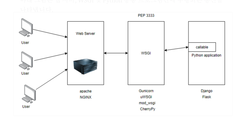
코드를 읽기 전에 먼저 대략적인 개념들을 잡고가는 것이 도움이 될 것 같습니다. Flask는 Web 개발에 사용되는 프레임워크이며, WSGI(Web Server Gateway Interface)라는 통신규격을 지키고 있습니다. 이는 기존의 웹서버와 웹 애플리케이션 간의 제약사항을 허물어 주면서, 각각의 역할에 따라서 동작할 수 있도록 하였습니다.

images

출처: https://medium.com/analytics-vidhya/what-is-wsgi-web-server-gateway-interface-ed2d290449e

이렇게 구조를 가져가면서 얻을 수 있는 장점은 주로 1) 성능 향상2) 확장성 에 있습니다. 이 포스트에서는 코드를 읽는 것이 주이므로, 간단하게만 언급하고 넘어가도록 하겠습니다.

위 인터페이스의 규격은 아래의 코드로 확인할 수 있습니다. Request 라는 Callable Object 를 Web Application에서 받아서 Response 라는 결과를 반환하는 것입니다.
(아래의 예제 코드의 werkzeugflask 의 코어가 되는 라이브러리로, 같은 개발자가 만들었습니다.)

from werkzeug.wrappers import Request, Response

@Request.application
def application(request):
    return Response('Hello, World!')

if __name__ == '__main__':
    from werkzeug.serving import run_simple
    run_simple('localhost', 4000, application)

The Pallets Projects

현재 flask는 The Pallets Projects 라는 Organization에서 관리가 되고 있습니다. 이 페이지에 들어가 보시면, 사용해봤을 법한 몇가지 유명한 라이브러리들이 같이 만들어졌음을 알 수 있습니다.

  • click : Command Line Interface Creation Kit 의 약자로서, 간단하게 cli 를 조작할 수 있습니다. (10.6k Star)
  • jinja : HTML 템플릿 엔진으로, 다양한 기능들과 Python과 비슷한 syntax 그리고 데이터 연결이 가능하게 해줍니다. (7.6k Star)
  • werkzeug : WSGI Web 개발에 핵심이 되는 라이브러리 (5.7k Star)

위의 3가지 프로젝트가 대표적이죠. flask 뿐만 아니라, 어디선가 봤던 유명한 라이브러리들이 포함되어 있다는 것이 신기하였습니다. 또한 이 모든 프로젝트들이 Armin Ronacher 에 의해서 만들어졌다는 것 입니다. 개발자들의 생산성은 개개인마다 굉장히 차이가 크다는 것은 실험 결과를 통해 입증되었지만, 이렇게 개인이 만든 라이브러리들이 전세계적으로 사용되는 것을 보면 참 대단하다는 생각이 듭니다.

만든이가 동일한 사람이기 때문에, 라이브러리의 성격들이 비슷하다. click과 flask를 보면, 사용성에 초점이 확 맞춰져 있는 것을 느낄 수 있다. 위 모든 프로젝트에 들어가있는 A Simple Example 을 보면 확인할 수 있는 점이기도 합니다.

Flask

(Flask 의 코드는 ‘1.1.2’ Tag를 기준으로 살펴봅니다.)

위에서 살펴본 것처럼, Flask는 The Pallets Projects의 다양한 라이브러리를 통해서 이루어져 있습니다. 간단하게는 werkzeug를 감싸서 만든 Web Application Framework 라고 할 수 있습니다.

install_requires=[
    "Werkzeug>=0.15",
    "Jinja2>=2.10.1",
    "itsdangerous>=0.24",
    "click>=5.1",
],

디자인 철학

프레임워크는 전반적으로 단순함을 기초로 하고 있습니다. 의존성을 최소로 하고 있는데, 흔히 Web 개발에 사용되는 DB 또한 내장되어 있지 않고 (Django는 postgreSQL을 기본으로 사용하도록 되어있습니다.) 최소한으로 템플릿은 사용하므로 위의 Jinja2를 템플릿 엔진으로 의존하고 있는 정도입니다. 확장은 사용자에게 달려있는 것이죠.

그리고 명시적인 Application 객체를 사용하고 있습니다. 여기에 대해서는 다음 3가지 이유가 있습니다.

  1. 암시적인 Application 객체가 한 번에 하나의 인스턴스만 있어야 한다는 것.
  2. 패키지 이름과 연동하여 리소스 할당.
  3. 일반적으로 명시적인 것이 암묵적인 것보다 낫기 때문.

만약에 명시적인 Application 객체를 사용하지 않으면, 아래와 같은 코드가 될 것 입니다.

from hypothetical_flask import route

@route('/')
def index():
    return 'Hello World!'

Application의 범주를 정의하는 것이 모호할 것이며, 하나의 객체에 여러개의 application이 동작하면서 혼동을 줄 수도 있을 것 입니다. 그리고 명시적인 Application 객체는 최소한으로 기능을 할당해서 Unit test도 진행할 수 있는 장점이 있다고 저자는 말하고 있습니다.

Code

코드는 전반적으로 함수와 객체가 역할에 맞춰서 잘 나뉘어 있으며, Python 언어가 제공하는 기본 기능들을 최대한 활용하여 (Pythonic한), 가독성에 굉장히 신경을 쓴 것을 코드 전반적으로 느낄 수 있습니다. 다음은 몇가지 세부 코드들은 들어가서 살펴보겠습니다.

helpers.py : 다양한 유틸 함수 및 클래스를 선언

# https://github.com/pallets/flask/blob/1.1.2/src/flask/helpers.py

def get_env():
    """Get the environment the app is running in, indicated by the
    :envvar:`FLASK_ENV` environment variable. The default is
    ``'production'``.
    """
    return os.environ.get("FLASK_ENV") or "production"

def get_debug_flag():
    """Get whether debug mode should be enabled for the app, indicated
    by the :envvar:`FLASK_DEBUG` environment variable. The default is
    ``True`` if :func:`.get_env` returns ``'development'``, or ``False``
    otherwise.
    """
    val = os.environ.get("FLASK_DEBUG")

    if not val:
        return get_env() == "development"

    return val.lower() not in ("0", "false", "no")

def url_for(endpoint, **values):
    ...

def get_template_attribute(template_name, attribute):
    ...

def total_seconds(td):
    """Returns the total seconds from a timedelta object.
    :param timedelta td: the timedelta to be converted in seconds
    :returns: number of seconds
    :rtype: int
    """
    return td.days * 60 * 60 * 24 + td.seconds

위 코드들에서 확인할 수 있는 것처럼, 자주 사용하는 유틸리티성의 함수들이 직관적인 네이밍과 docstring과 함께 작성이 되어있습니다. docstring 에는 입력에 대한 type과 출력에 대한 type 또한 명시가 되어있습니다. 이 부분들은 Python 3.5 버전부터 추가된 typing 라이브러리를 활용하는 것도 가능하겠네요.

  • templating.py : Jinja2를 통해서 템플릿 랜더링 (코드 작성 방식)

이 부분은 템플릿 엔진이 동작하는 로직을 담고 있습니다. 여기서 다루고자 하는 부분은 코드의 작성 방식입니다. «클린코드» 에서는 코드를 위에서 아래로 보는, 신문 기사에 비유를 합니다. 먼저 핵심 요약을 위에서 다루고, 아래에서 세부적인 내용들을 다루는 것 입니다.

def get_source(self, environment, template):
    if self.app.config["EXPLAIN_TEMPLATE_LOADING"]:
        return self._get_source_explained(environment, template)
    return self._get_source_fast(environment, template)

def _get_source_explained(self, environment, template):
    ...

def _get_source_fast(self, environment, template):
    ...

Flask 역시 위에서 아래로 읽을 수 있도록 코드가 작성되어 있고, 객체지향에서 접근권한을 명시하는 방식 또한 적용되어 있는 것을 보실 수 있습니다. Python은 코드차원에서 이를 지원하지는 않지만, 암묵적인 규칙이 있습니다.

def method_name(): # public
def _method_name():  # protected or private
def __method_name(): # private

wrappers.py : werkzeug 를 감싸서 객체 선언 (객체의 확장방식)

이 코드에서는 1편 PyTorch의 Function의 객체의 확장과 거의 같은 방식을 보실 수 있습니다.

# https://github.com/pallets/flask/blob/1.1.2/src/flask/wrappers.py

from werkzeug.wrappers import Request as RequestBase
from werkzeug.wrappers import Response as ResponseBase

class JSONMixin(_JSONMixin):
    ...

class Request(RequestBase, JSONMixin):
    ...

class Response(ResponseBase, JSONMixin):
    ...

바로 Base 객체를 두고 Mixin 을 통해서 인터페이스 및 속성을 확장해 나가는 방식입니다. (이 Mixin에 대해서는 1편 PyTorch 에서 간단하게 설명하고 있습니다.)

한가지 재미있는 점은 Mixin 뿐만 아니라, Meta Class를 활용하는 방식 또한 PyTorch에서 봤던 것과 동일합니다.

# https://github.com/pallets/flask/blob/1.1.2/src/flask/_compat.py#L60

def with_metaclass(meta, *bases):
    """Create a base class with a metaclass."""
    # This requires a bit of explanation: the basic idea is to make a
    # dummy metaclass for one level of class instantiation that replaces
    # itself with the actual metaclass.
    class metaclass(type):
        def __new__(metacls, name, this_bases, d):
            return meta(name, bases, d)

    return type.__new__(metaclass, "temporary_class", (), {})

with_metaclass 는 객체의 빌트인 함수들의 동작을 바꿔서, 원하는 방식대로 동작하는 객체를 만드는 데 사용이 됩니다. PyTorch에서 Function 객체를 위 메서드를 통해서 정의하고 있죠. (자세한 것은 1편을 참고해주세요.) 프로젝트 시기상 Flask가 훨씬 먼저 만들어지고, 이후에 PyTorch가 만들어졌기 때문에.. PyTorch의 메인테이너들은 Flask의 코드스타일을 비슷하게 따라갔고 몇가지 그대로 사용하는 케이스도 있었던 것으로 생각이 됩니다. Flask의 코드들이 가독성이 좋고 사용성 또한 직관적이였던 것처럼, PyTorch 역시 그럴마한 이유가 있었네요.

signals.py : Application이 동작하는 시그널을 감지

# https://github.com/pallets/flask/blob/1.1.2/src/flask/signals.py#L54

# Core signals.  For usage examples grep the source code or consult
# the API documentation in docs/api.rst as well as docs/signals.rst
template_rendered = _signals.signal("template-rendered")
before_render_template = _signals.signal("before-render-template")
request_started = _signals.signal("request-started")
request_finished = _signals.signal("request-finished")
request_tearing_down = _signals.signal("request-tearing-down")
got_request_exception = _signals.signal("got-request-exception")
appcontext_tearing_down = _signals.signal("appcontext-tearing-down")
appcontext_pushed = _signals.signal("appcontext-pushed")
appcontext_popped = _signals.signal("appcontext-popped")
message_flashed = _signals.signal("message-flashed")

이 부분은 동작에 대한 신호를 판별하는 부분으로, 거의 유일하게 Python의 내장 라이브러리와 자신이 만든 라이브러리를 제외하고 다른 사람이 만든 것을 활용하고 있습니다. 그리고 그 마저도 꼭 필요한 dependency는 아니기도 합니다.

라이브러리를 개발할때, 필요하다면 이와 같이 Blinker 라는 dispatching system을 사용할 수 있을 것 같습니다.

**werkzeug/datastructures.py** : (번외로) werkzeug 에서 유틸리티처럼 정의한 데이터구조 클래스들

이번 Flask 코드를 살펴보면서 자연스럽게 연결되어 있는 라이브러리에 대해서도 살짝 살펴보게 되었습니다. 그 중에서 한가지 참고하기에 가장 좋다고 생각되는 코드를 소개시켜드리고자 합니다.

# https://github.com/pallets/werkzeug/blob/1.0.1/src/werkzeug/datastructures.py

class ImmutableListMixin:
    ...

class ImmutableList(ImmutableListMixin, list):
    ...

class OrderedMultiDict(MultiDict):
   ...

    def __eq__(self, other):
        ...

    def __getstate__(self):
        ...

    def __setstate__(self, values):
        ...

위와 같은 방식으로 Mixin을 정의해서 필요한 데이터구조를 확장하기도 하고, 기본으로 사용하는 생성자 __init__ 이외에도 __eq__, __ne__, __getstate__, __setitem__, items, pop 등의 기본 내장되어 있는 Built-in 함수들을 필요에 맞춰서 재구현한 것들을 볼 수 있습니다.

# https://github.com/pallets/werkzeug/blob/1.0.1/src/werkzeug/datastructures.py#L919

class Headers(object):
    """An object that stores some headers.  It has a dict-like interface
    but is ordered and can store the same keys multiple times.
    This data structure is useful if you want a nicer way to handle WSGI
    headers which are stored as tuples in a list.
    ...
    """

Request에 사용되는 Headers 또한 기본 Built-in 함수들을 직관적으로 사용할 수 있도록 재구현이 되어 있습니다. 이 코드들을 보다보니, PyTorch의 Module 클래스가 생각나기도 하네요!

그 외에도 다양하게 decorator가 구현되고 직관적으로 사용되는 점들도 있으니, 코드를 살펴보시면서 참고하시면 좋겠습니다. (@setupmethod 예시)

끝으로

이번에 Flask를 살펴보면서.. 한명의 개인이 전 세계적으로 사용되는 다양한 오픈소스를 만들어내는 것도 신기하였고, 좋은 코드를 읽는데 있어서 Flask를 추천하는 것이 이해가 되었습니다. Pythonic한 코드스타일의 정말 좋은 표본이라고 생각하고 앞으로도 많이 참고를 하게 될 것 같습니다.

그리고 위에서 PyTorch가 Flask에 영향을 정말 많이 받은 만큼, Flask를 먼저 살펴보고 PyTorch로 넘어가는 것도 괜찮았을 것 같네요!

References

Categories
Offsites

How (and why) to raise e to the power of a matrix | DE6

Categories
Offsites

위대한 제품을 만드는 모두를 위한, 창의성을 지휘하라

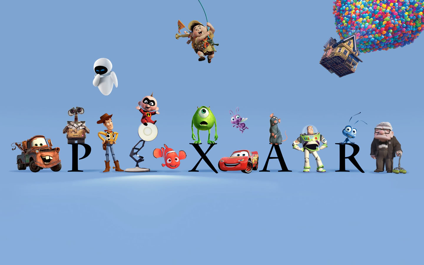
픽사 애니메이션 스튜디오는 아래 이미지에서 낯익은 케릭터들이 많이 있는 만큼, 흥행한 작품들이 굉장히 많은 회사 입니다. 특히 초창기에는 작품을 낼때마다 박스오피스 1위를 할 정도였죠. 어떻게 애니메이션을 만드는지 아는 것이 별로 없지만, 창의성이 중요하다는 것은 알 수가 있습니다. 이런 창의성이 요구되는 활동을 성공적으로, 그리고 꾸준하게 해낼 수 있었던 비결은 무엇일까요?

image.png

출처: https://www.creativebloq.com/animation/job-at-pixar-10121018

그에 대한 답의 일부가 아래 애드 캣멀이 지은 ≪창의성을 지휘하라≫ 에 담겨있습니다.

이 책에는 저자 애드 캣멀이 픽사라는 회사와 함께 성장하는 과정과 애니메이션을 하나하나 성공시켜가면서, 경영자로서 스스로 무수히 많은 질문을 던지고 답을 찾아가는, 이러한 전반적인 과정들이 담겨있습니다. 그 뿐만 아니라 실질적으로 참고할 수 있도록, 픽사에서 실제 진행한 프로세스들에 대한 이야기도 포함되어 있습니다.

image.png

출처: https://www.aladin.co.kr/shop/wproduct.aspx?ItemId=45834844

경영자로서의 애드 캣멀

저는 이 책을 읽으면서 특히 저자가 경영자로서 계속해서 마주치는 문제들에 대해서 다양한 관점으로 고려하면서 답을 찾아가는 과정이 인상이 깊었습니다. 숫자를 세어본 적은 없지만, 계속해서 물음표로 글이 이어지는 부분들도 적지 않았던 것 같네요.

픽사 사장으로서 내 목표는 언제나 픽사가 창업자들(스티브 잡스, 존 래스터, 그리고 나)보다 오래 생존할 수 있게 픽사에 계속 생명력을 불어놓는 창의적 기업문화를 구축하는 것이었다. 예술과 상업이라는 상호충돌하면서도 상호보완적인 동력을 관리하느라 애를 먹고 있는 경영자들과 창의적 기업문화에 관한 철학을 공유하는 것도 내 목표다. … 나는 어떤 분야에든 사람들이 창의성을 발휘해 탁월한 성과를 내도록 이끄는 훌륭한 리더십이 필요하다고 생각한다.

  • 머리말 – 잃어버리고 되찾은 것 중에서

경영이란 이런 것이다. 타당한 이유에 따라 내린 결정이 새로운 문제를 초래하고, 이 새로운 문제를 해결하기 위해 또 다른 결정을 내려야 한다. 기업에서 발생하는 문제는 최초의 오류를 수정하는 것마으로 간단히 풀리는 법이 없다. 하나의 문제를 해결하는 일은 여러 단계를 거쳐야 하는 과정이다. 최초의 문제뿐만 아니라 여기서 파생된 문제가 무엇인지 파악해 함께 해결해야 한다.

  • Chapter 1 애니메이션과 기술의 만남

나는 오랫동안 인식의 한계에 대해 고민했다. 경영자는 항상 인식의 한계에 관한 문제로 인해 고민하게 마련이다. 우리는 어디까지 볼 수 있는가? 얼마나 많은 것을 불명확하게 인식하고 있는가? 우리가 카산드라의 경고를 무시하고 있는 건 아닐까? 다시 말해, 우리가 최선을 다해 문제를 파악하려고 노력해도 문제를 인식하지 못하는 저주를 받은 것은 아닐까? 이런 의문들의 답을 찾는 과정은 창의적 기업문화를 유지하는 열쇠다. 그리고 그 답을 탐구하는 것이 이 책의 핵심 내용이다.

  • Chapter 9 잠재적 위험에 대처하는 법 중에서

이 부분은 애드 캣멀이 어떠한 사람인지를 알 수 있는 대목이기도 합니다.

나는 다른 기업 사람들이 나와 달리 공격적이고 확신에 찬 행동을 하는 것을 보고, 내가 사장답지 않아 보일까 봐 걱정했다. 더 정확히 말하면, 나는 실패가 두려웠다.
나는 연설에서 8~9년 전에야 겨우 내가 사기꾼이 된 것 같은 기분에서 벗어날 수 있었다고 털어놨다. … “자신이 사기꾼처럼 느껴지는 분이 있나요?” 그러면 언제나 모든 직원이 손을 든다.
… 자신이 경영자로서 잘해 나가고 있는지 파악하려면, 머릿속에서 경영자란 어떤 것이어야 한다는 심성모형을 지워야 한다. 경영자의 성공을 측정하는 척도는 ‘팀원들이 잘 협력해 핵심적인 문제들을 해결하고 있는가?’ 이다.

  • Chapter 6 실패와 공포에 대처하는 법 중에서

제품을 만드는 모두를 위한,

이 책을 추천하는 이유는 픽사라는 회사를 가지고 이야기를 하고 있지만, 제품을 만드는 수 많은 회사들에도 적용할 수 있는 좋은 길잡이이기 때문입니다.

먼저 우리는 그 어느때보다 ‘창의력’이 중요시 되는 시대에 살고 있습니다. ‘지식근로자’라는 말은 1968년 피터드러커가 ≪단절의 시대≫ 을 저술하면서 처음 언급 했었습니다. 이제는 이 지식근로자라는 말이 전혀 낯설지 않은 시대에 우리는 살고 있습니다. 또한 실제로 AI가 급격히 발전하면서 단순 반복적인 일들이 대체되고 있는 상황입니다. 이에 자연스럽게, AI가 잘하지 못하는 일들이 이 지식근로자들에게 요구되고 있습니다. 이러한 일들 중 가장 기본이 되는 것이 무엇일까요? 핵심 요소 중에서 하나가 바로 창의성일 것입니다.

새로운 제품을 만드는데 있어서 이 창의성은 굉장히 중요한 요소입니다. 문제를 발견하고, 어떤 식으로 풀지 이 전반적인 과정에 모두 이 창의성이 활용되기 때문이죠. 그리고 픽사에서 애니메이션을 제작하는 것을 스타트업에서 제품을 만들어내는 것에 비유할 수 있습니다. 흔히 스타트업에서 새로운 제품을 만드는 과정을 다음과 같이 이야기 할 수 있습니다.

  • 고객을 깊이 이해하고, 주어진 문제를 풀어내서, 고객에게 전달하여 감동을 주는 것.

에니메이션을 만드는 과정 또한 비슷한 프레임을 가지고 있습니다.

  • 전달하고자 하는 스토리를 구상하고, 배경과 하나하나의 케릭터에 숨을 불어넣어서, 관객들에게 전달하여 감동을 주는 것.

전달하는 제품의 형태만 다를 뿐, 고객(관객)들에게 감동을 주는 것은 동일하기 때문입니다. 그럼 이 다음부터는 픽사가 어떤 식으로 성장해왔는지 간략하게 다뤄보겠습니다.

픽사의 정체성, 목표와 기업문화 (사람과 프로세스)

먼저 인상 깊었던 부분들 중 하나는 픽사라는 회사의 색깔을 명확하게 한 것입니다. 다음은 회사의 정체성을 구축하는 데 있어 가장 중요한 두가지 요소입니다. 첫 번째가 회사가 추구하는 목표(미션)가 무엇인지, 두 번째로는 기업 문화에 해당합니다. 픽사는 사람들에게 감동을 주는 애니메이션을 만드는 것을 목표로 하였고, 상황에 타협하지 않았고 본질을 계속 추구한 집단이기도 하였습니다.

당시 픽사는 파산 위기에 처한 신생 영화사에 불과했지만, 직원들은 신념을 공유했다. 우리가 보고 싶은 영화를 만들면 관객들도 보러 올 것이라는 신념이었다. 우리는 이 신념을 지키기 위해, 계속해서 커다란 바위를 산꼭대기로 밀어올리는 시시포스처럼 불가능한 일에 무모하게 도전하는 기분을 맛봐야 했다.
… 픽사 임직원이 자부심을 느낀 대목은 이런 숫자가 아니다. 수익은 기업의 성과를 측정하는 여러 가지 잣대 중 하나로, 가장 의미 있는 잣대라고 할 수 없다. 내가 가장 자부심을 느끼는 부분은 우리가 만든 작품의 예술적 성취도다. … 우리가 추구한 진짜 목적은 그때나 지금이나 위대한 영화를 제작하는 것이다.

  • 머리말 – 잃어버리고 되찾은 것 중에서

‘토이 스토리’를 제작하는 과정에서 픽사에 지대한 영향을 미치게 될 두 가지 창작 원칙이 만들어졌다. …
제1원칙은 “스토리가 왕이다(Story is King)” 이다. …
제2원칙은 “프로세스를 신뢰하라(Trust the Process)”다. 우리는 이 원칙을 좋아했다. 제작 과정의 고민을 덜어주는 원칙이기 때문이다.

  • Chapter 4 픽사의 정체성 구축 중에서

우리는 디즈니 중역들을 만나 극장용보다 질이 낮은 비디오 대여용 애니메이션을 제작하는 일은 픽사의 기업 성향에 맞지 않는다고 말했다. 픽사의 기업문화는 이를 용납하지 못했다. 우리는 진로를 바꾸어 ‘토이 스토리2’를 극장용 애니메이션으로 만들자고 제안했다. 놀랍게도 디즈니 중역들은 흔쾌히 승낙했다.

  • Chapter 4 픽사의 정체성 구축 중에서

기업문화에 있어서 가장 중요한 요소는 ‘사람’ 입니다. 많은 책들에서 적합한 사람, 인재밀도 등을 언급하는 것처럼, 저자 역시 사람에 대해서 특히 중요하게 여기는 것을 볼 수가 있습니다.

나는 다음과 같은 교훈을 얻었다. 좋은 아이디어를 평범한 팀에 맡기면 실망스러운 결과가 나온다. 반면 평범한 아이디어를 탁월한 팀에 맡기면, 그들은 아이디어를 수정하든 폐기하든 해서 더 나은 결과를 내놓는다.
이 교훈은 더 설명할 가치가 있다. 적합한 팀에게 일을 맡기는 것이 아이디어를 성공적으로 구현하는 선결 조건이다. 재능 있는 인재들을 원한다고 말하기는 쉽고, 경영자들 또한 재능 있는 인재들을 원하지만, 정말로 핵심 관건은 이런 인재들이 상호작용하는 방식이다. 아무리 영리한 사람들을 모아놓아도 서로 어울리지 않으면 비효율적인 팀이 된다. 경여앚가 직원 개개인의 재능이 아니라 팀이 돌아가는 상황에 초점을 맞추는 편이 낫다는 뜻이다. 좋은 팀은 서로 보완해주는 사람들로 구성된다. … 업무에 적합한 인재들이 상성이 맞는 사람들과 함께 일하도록 하는 것이 좋은 아이디어를 내는 것보다 중요하다.

  • Chapter 4 픽사의 정체성 구축 중에서

한 사람만이 내가 던진 질문에 오류가 있다고 지적했다. 아이디어는 사람에게서 나온다. 사람이 없으면 아이디어도 없다. 따라서 사람이 아이디어보다 중요하다.
왜 사람이 아이디어보다 중요하다고 생각하지 못할까? 너무나 많은 사람이 아이디어가 사람들과 완전히 분리된 채 독립적으로 형성되고 존재한다고 착각하기 때문이다. 아이디어는 독립적인 존재가 아니다. 아니디어는 종종 수십 명이 관여하는 수만 가지 의사결정을 통해 형성된다. … 영화는 하나의 아이디어만으로 만들어질 수 없다. 영화는 여러 아이디어의 집합체다. 이런 아이디어들을 구상하고 현실로 구현하는 것은 결국 사람이다. 모든 제품이 마찬가지다. …
다시 말해, 사람(직원들의 근무 습관, 재능, 가치)에게 초점을 맞추는 것이 모든 창조적 사업의 핵심 성공 비결이다. 제작 과정에서 나는 이런 사실을 이전보다 명확히 인식하게 됐다. .. 이후 픽사는 사람을 우선하는 경영 모델을 꾸준히 실천하고 있다. 세부적인 수정은 있었지만, 근본 원리는 언제나 같다. 좋은 인재를 육성하고 지원하면 그들이 좋은 아이디어를 내놓는다는 것이다.토이>

  • Chapter 4 픽사의 정체성 구축 중에서

다음으로는 뛰어난 사람들이 각자의 역량을 펼칠 수 있도록, 서로 효율적으로 협력하는 방법들에 대한 고민을 계속 하는 것을 볼 수 있습니다. 이는 제품의 질이 직원들에게 달려있다는 것을 전적으로 믿기 때문이죠.

당시 일본 제조업에서 일어난 품질관리 혁명을 설명하기 위해 적기공급생산(just-in-time manufacturing), 전사적 품질관리(total quality control) 같은 경영학 용어들이 나왔다. 이런 용어들이 설명하려는 아이디어는 간단하다. 즉, 문제를 파악해 수정할 권한을 고위 간부부터 생산라인 말단직원까지 모든 임직원에게 부여해야 한다는 것이다. 에드워드 데밍은 어떤 직급의 직원이라도 제조 과정에서 문제를 발견하면 조립라인을 멈추도록 장려해야 한다고 생각했다. …
에드워드 데밍과 도요타의 접근법은 제품 생산 과정에 밀접하게 관여하는 사람들에게 제품의 품질을 높일 권한과 책임을 부여했다. 이 과정에서 일본 근로자들은 자신이 단지 컨베이어벨트 위를 지나가는 부품들을 조립하는, 영혼 없는 톱니바퀴 같은 존재가 아니라, 제품 생산 과정의 문제를 지적하고, 변화를 제안하고, 문제 해결에 기여해 회사를 키우는 구성원이라는 ‘자부심’을 느꼈다(나는 특히 마지막 대목이 중요하다고 생각한다).
… 에드워드 데밍의 품질관리 이론은 ‘모든 직원은 먼저 허락받지 않은 채, 문제 해결에 나설 수 있어야 한다’ 라는 민주적 원칙에 기반을 두고 있다. … 경영진이 단기이익 극대화에 집착하자 자부심을 가지고 품질 향상에 힘쓰던 직원들은 영혼을 잃은 채 일하게 됐고, 그 결과 품질 결함이 발생하기 시작했다.

  • Chapter 3 의 탄생과 목표의 재정립 중에서토이>

이러한 고민들의 결과로서 창작 제 2원칙으로 “프로세스를 신뢰하라” 가 있는 것처럼, 픽사에서는 좋은 작품을 만들기 위한 다양한 프로세스를 정립하기 위한 많은 시도들이 있었습니다. 아래는 픽사라는 회사가 어느정도 큰 큐모를 갖춘 이후에 정립된 프로세스을 나열해둔 것 입니다.

  1. 데일리스 회의
  2. 현장답사
  3. 한도 결정
  4. 기술과 예술의 융합
  5. 소규모 실험
  6. 보는 법 배우기
  7. 사후분석 회의
  8. 픽사대학

프로세스들을 하나하나 보다보면, 이러한 생각이 들기도 합니다. ‘우리도 이런 것들은 하고 있는 거 같은데?’ 하지만 자세히 들여다보면 픽사가 구축해온 기업문화를 기반으로 위 프로세스들이 일반적인 기업들과는 다르게 돌아가는 것을 이해할 수 있습니다. 최근에 읽었던 넷플릭스의 ≪규칙없음≫ 에서 자유와 책임이 주어지는 것처럼, 픽사에서 역시 개개인에게 자유와 책임이 주어지는 것을 느낄 수 있었습니다.

‘픽사의 브레인트러스트가 다른 기업의 피드백 매커니즘과 다른 게 뭐야?’ … 첫째, 픽사의 브레인트러스트는 스토리텔링을 심도 있게 이해하는 사람들, 대게 작품 제작에 참여해본 경험이 있는 사람들로 구성된다. 픽사 감독들은 다양한 사람들의 비평을 환영하지만(사실 모든 픽사 직원들은 중간결과물을 보고 의견서를 보내야 한다), 특히 동료 감독, 각본가가 보낸 피드백을 더 진지하게 받아들인다. 둘째, 픽사의 브레인트러스트는 지시할 권한이 없다. 이는 중요한 차이다. 감독은 브레인트러스트의 특정 제안을 꼭 받아들여야 할 필요가 없다. 브레인트러스트 회의 후, 브레인트러스트의 피드백을 어떻게 받아들일지 결정하는 것은 감독의 몫이다.

  • Chapter 5 솔직함의 가치 중에서

위의 프로세스 외에도 인턴 프로그램, 전사 워크샵인 노트 데이 등에 대한 이야기가 담겨 있습니다. 특히 노트데이에서는 단순히 직원들의 참여를 유도하는 것이 아니라 토론회가 제대로 돌아갈 수 있도록 설계하는 과정까지 담겨 있어서 흥미롭게 볼 수 있었습니다.

제작비를 10퍼센트 감축하는 방안을 고민하는 자리에서 귀도 쿼로니는 간단한 제안을 했다.
“모든 직원에게 비용 삭감 아이디어를 내달라고 요청합시다.”
존 래스터는 흥분한 얼굴로 말했다. “흥미로운 제안이군요. 하루 동안 모든 픽사 직원의 업무를 중단하고, 이 문제를 해결할 방안을 얘기해보는 게 어떨까요?”

  • Chapter 13 노트 데이 토론회 중에서

끝으로

수 많은 스타트업을 꿈꾸는 분들에게, 특히 정체성이 명확한 회사를 만들고 싶은 분들에게 좋은 길잡이가 되어줄 책이라고 생각을 합니다. 마지막으로 존 래스터가 기업문화에 대해서 이야기한 문장과 애드 캣멀의 경영자의 목표로 책 소개를 마무리 하고자 합니다.

존 래스터는 종종 픽사의 조직문화를 살아 있는 유기체에 비유했다. “지구상에 출현한 적 없는 새로운 생명체를 키우는 방법을 우리가 발견한 것 같아요.”

이 책을 써내려오면서 내 목표는 픽사와 디즈니 애니메이션 스튜디오 직원들이 어떻게 얼마나 끈질기게 비전을 실현할 방법을 모색했는지 독자들에게 알리는 것이었다. 미래는 목적지가 아니라 방향이다. 우리가 할 일은 현재의 진로가 옳은지 매일 점검하고, 길을 벗어났다면 방향을 수정하는 것이다. … 불확실성과 변화는 변수가 아니라 인생에서 피할 수 없는 상수다. 불확실성과 변화가 있기에 인생이 재미있는 것이다.

원래 경영자의 목표는 달성하기 쉬울 수 없다. 경영자의 목표는 탁월한 제품을 만드는 것이다.

Categories
Offsites

Constructing Transformers For Longer Sequences with Sparse Attention Methods

Natural language processing (NLP) models based on Transformers, such as BERT, RoBERTa, T5, or GPT3, are successful for a wide variety of tasks and a mainstay of modern NLP research. The versatility and robustness of Transformers are the primary drivers behind their wide-scale adoption, leading them to be easily adapted for a diverse range of sequence-based tasks — as a seq2seq model for translation, summarization, generation, and others, or as a standalone encoder for sentiment analysis, POS tagging, machine reading comprehension, etc. The key innovation in Transformers is the introduction of a self-attention mechanism, which computes similarity scores for all pairs of positions in an input sequence, and can be evaluated in parallel for each token of the input sequence, avoiding the sequential dependency of recurrent neural networks, and enabling Transformers to vastly outperform previous sequence models like LSTM.

A limitation of existing Transformer models and their derivatives, however, is that the full self-attention mechanism has computational and memory requirements that are quadratic with the input sequence length. With commonly available current hardware and model sizes, this typically limits the input sequence to roughly 512 tokens, and prevents Transformers from being directly applicable to tasks that require larger context, like question answering, document summarization or genome fragment classification. Two natural questions arise: 1) Can we achieve the empirical benefits of quadratic full Transformers using sparse models with computational and memory requirements that scale linearly with the input sequence length? 2) Is it possible to show theoretically that these linear Transformers preserve the expressivity and flexibility of the quadratic full Transformers?

We address both of these questions in a recent pair of papers. In “ETC: Encoding Long and Structured Inputs in Transformers”, presented at EMNLP 2020, we present the Extended Transformer Construction (ETC), which is a novel method for sparse attention, in which one uses structural information to limit the number of computed pairs of similarity scores. This reduces the quadratic dependency on input length to linear and yields strong empirical results in the NLP domain. Then, in “Big Bird: Transformers for Longer Sequences”, presented at NeurIPS 2020, we introduce another sparse attention method, called BigBird that extends ETC to more generic scenarios where prerequisite domain knowledge about structure present in the source data may be unavailable. Moreover, we also show that theoretically our proposed sparse attention mechanism preserves the expressivity and flexibility of the quadratic full Transformers. Our proposed methods achieve a new state of the art on challenging long-sequence tasks, including question answering, document summarization and genome fragment classification.

Attention as a Graph
The attention module used in Transformer models computes similarity scores for all pairs of positions in an input sequence. It is useful to think of the attention mechanism as a directed graph, with tokens represented by nodes and the similarity score computed between a pair of tokens represented by an edge. In this view, the full attention model is a complete graph. The core idea behind our approach is to carefully design sparse graphs, such that one only computes a linear number of similarity scores.

Full attention can be viewed as a complete graph.

Extended Transformer Construction (ETC)
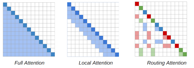
On NLP tasks that require long and structured inputs, we propose a structured sparse attention mechanism, which we call Extended Transformer Construction (ETC). To achieve structured sparsification of self attention, we developed the global-local attention mechanism. Here the input to the Transformer is split into two parts: a global input where tokens have unrestricted attention, and a long input where tokens can only attend to either the global input or to a local neighborhood. This achieves linear scaling of attention, which allows ETC to significantly scale input length.

In order to further exploit the structure of long documents, ETC combines additional ideas: representing the positional information of the tokens in a relative way, rather than using their absolute position in the sequence; using an additional training objective beyond the usual masked language model (MLM) used in models like BERT; and flexible masking of tokens to control which tokens can attend to which other tokens. For example, given a long selection of text, a global token is applied to each sentence, which connects to all tokens within the sentence, and a global token is also applied to each paragraph, which connects to all tokens within the same paragraph.

An example of document structure based sparse attention of ETC model. The global variables are denoted by C (in blue) for paragraph, S (yellow) for sentence while the local variables are denoted by X (grey) for tokens corresponding to the long input.

With this approach, we report state-of-the-art results in five challenging NLP datasets requiring long or structured inputs: TriviaQA, Natural Questions (NQ), HotpotQA, WikiHop, and OpenKP.

Test set result on Question Answering. For both verified TriviaQA and WikiHop, using ETC achieved a new state of the art.

BigBird
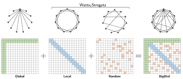
Extending the work of ETC, we propose BigBird — a sparse attention mechanism that is also linear in the number of tokens and is a generic replacement for the attention mechanism used in Transformers. In contrast to ETC, BigBird doesn’t require any prerequisite knowledge about structure present in the source data. Sparse attention in the BigBird model consists of three main parts:

  • A set of global tokens attending to all parts of the input sequence
  • All tokens attending to a set of local neighboring tokens
  • All tokens attending to a set of random tokens
BigBird sparse attention can be seen as adding few global tokens on Watts-Strogatz graph.

In the BigBird paper, we explain why sparse attention is sufficient to approximate quadratic attention, partially explaining why ETC was successful. A crucial observation is that there is an inherent tension between how few similarity scores one computes and the flow of information between different nodes (i.e., the ability of one token to influence each other). Global tokens serve as a conduit for information flow and we prove that sparse attention mechanisms with global tokens can be as powerful as the full attention model. In particular, we show that BigBird is as expressive as the original Transformer, is computationally universal (following the work of Yun et al. and Perez et al.), and is a universal approximator of continuous functions. Furthermore, our proof suggests that the use of random graphs can further help ease the flow of information — motivating the use of the random attention component.

This design scales to much longer sequence lengths for both structured and unstructured tasks. Further scaling can be achieved by using gradient checkpointing by trading off training time for sequence length. This lets us extend our efficient sparse transformers to include generative tasks that require an encoder and a decoder, such as long document summarization, on which we achieve a new state of the art.

Summarization ROUGE score for long documents. Both for BigPatent and ArXiv datasets, we achieve a new state of the art result.

Moreover, the fact that BigBird is a generic replacement also allows it to be extended to new domains without pre-existing domain knowledge. In particular, we introduce a novel application of Transformer-based models where long contexts are beneficial — extracting contextual representations of genomic sequences (DNA). With longer masked language model pre-training, BigBird achieves state-of-the-art performance on downstream tasks, such as promoter-region prediction and chromatin profile prediction.

On multiple genomics tasks, such as promoter region prediction (PRP), chromatin-profile prediction including transcription factors (TF), histone-mark (HM) and DNase I hypersensitive (DHS) detection, we outperform baselines. Moreover our results show that Transformer models can be applied to multiple genomics tasks that are currently underexplored.

Main Implementation Idea
One of the main impediments to the large scale adoption of sparse attention is the fact that sparse operations are quite inefficient in modern hardware. Behind both ETC and BigBird, one of our key innovations is to make an efficient implementation of the sparse attention mechanism. As modern hardware accelerators like GPUs and TPUs excel using coalesced memory operations, which load blocks of contiguous bytes at once, it is not efficient to have small sporadic look-ups caused by a sliding window (for local attention) or random element queries (random attention). Instead we transform the sparse local and random attention into dense tensor operations to take full advantage of modern single instruction, multiple data (SIMD) hardware.

To do this, we first “blockify” the attention mechanism to better leverage GPUs/TPUs, which are designed to operate on blocks. Then we convert the sparse attention mechanism computation into a dense tensor product through a series of simple matrix operations such as reshape, roll, and gather, as illustrated in the animation below.

Illustration of how sparse window attention is efficiently computed using roll and reshape, and without small sporadic look-ups.

Recently, “Long Range Arena: A Benchmark for Efficient Transformers“ provided a benchmark of six tasks that require longer context, and performed experiments to benchmark all existing long range transformers. The results show that the BigBird model, unlike its counterparts, clearly reduces memory consumption without sacrificing performance.

Conclusion
We show that carefully designed sparse attention can be as expressive and flexible as the original full attention model. Along with theoretical guarantees, we provide a very efficient implementation which allows us to scale to much longer inputs. As a consequence, we achieve state-of-the-art results for question answering, document summarization and genome fragment classification. Given the generic nature of our sparse attention, the approach should be applicable to many other tasks like program synthesis and long form open domain question answering. We have open sourced the code for both ETC (github) and BigBird (github), both of which run efficiently for long sequences on both GPUs and TPUs.

Acknowledgements
This research resulted as a collaboration with Amr Ahmed, Joshua Ainslie, Chris Alberti, Vaclav Cvicek, Avinava Dubey, Zachary Fisher, Guru Guruganesh, Santiago Ontañón, Philip Pham, Anirudh Ravula, Sumit Sanghai, Qifan Wang, Li Yang, Manzil Zaheer, who co-authored EMNLP and NeurIPS papers.

Categories
Offsites

sparklyr 1.6: weighted quantile summaries, power iteration clustering, spark_write_rds(), and more

Sparklyr 1.6 is now available on CRAN!

To install sparklyr 1.6 from CRAN, run

install.packages("sparklyr")

In this blog post, we shall highlight the following features and enhancements from sparklyr 1.6:

Weighted quantile summaries

Apache Spark is well-known for supporting approximate algorithms that trade off marginal amounts of accuracy for greater speed and parallelism. Such algorithms are particularly beneficial for performing preliminary data explorations at scale, as they enable users to quickly query certain estimated statistics within a predefined error margin, while avoiding the high cost of exact computations. One example is the Greenwald-Khanna algorithm for on-line computation of quantile summaries, as described in Greenwald and Khanna (2001). This algorithm was originally designed for efficient (epsilon)- approximation of quantiles within a large dataset without the notion of data points carrying different weights, and the unweighted version of it has been implemented as approxQuantile() since Spark 2.0. However, the same algorithm can be generalized to handle weighted inputs, and as sparklyr user @Zhuk66 mentioned in this issue, a weighted version of this algorithm makes for a useful sparklyr feature.

To properly explain what weighted-quantile means, we must clarify what the weight of each data point signifies. For example, if we have a sequence of observations ((1, 1, 1, 1, 0, 2, -1, -1)), and would like to approximate the median of all data points, then we have the following two options:

  • Either run the unweighted version of approxQuantile() in Spark to scan through all 8 data points

  • Or alternatively, “compress” the data into 4 tuples of (value, weight): ((1, 0.5), (0, 0.125), (2, 0.125), (-1, 0.25)), where the second component of each tuple represents how often a value occurs relative to the rest of the observed values, and then find the median by scanning through the 4 tuples using the weighted version of the Greenwald-Khanna algorithm

We can also run through a contrived example involving the standard normal distribution to illustrate the power of weighted quantile estimation in sparklyr 1.6. Suppose we cannot simply run qnorm() in R to evaluate the quantile function of the standard normal distribution at (p = 0.25) and (p = 0.75), how can we get some vague idea about the 1st and 3rd quantiles of this distribution? One way is to sample a large number of data points from this distribution, and then apply the Greenwald-Khanna algorithm to our unweighted samples, as shown below:

library(sparklyr)

sc <- spark_connect(master = "local")

num_samples <- 1e6
samples <- data.frame(x = rnorm(num_samples))

samples_sdf <- copy_to(sc, samples, name = random_string())

samples_sdf %>%
  sdf_quantile(
    column = "x",
    probabilities = c(0.25, 0.75),
    relative.error = 0.01
  ) %>%
  print()
##        25%        75%
## -0.6629242  0.6874939

Notice that because we are working with an approximate algorithm, and have specified relative.error = 0.01, the estimated value of (-0.6629242) from above could be anywhere between the 24th and the 26th percentile of all samples. In fact, it falls in the (25.36896)-th percentile:

pnorm(-0.6629242)
## [1] 0.2536896

Now how can we make use of weighted quantile estimation from sparklyr 1.6 to obtain similar results? Simple! We can sample a large number of (x) values uniformly randomly from ((-infty, infty)) (or alternatively, just select a large number of values evenly spaced between ((-M, M)) where (M) is approximately (infty)), and assign each (x) value a weight of (displaystyle frac{1}{sqrt{2 pi}}e^{-frac{x^2}{2}}), the standard normal distribution’s probability density at (x). Finally, we run the weighted version of sdf_quantile() from sparklyr 1.6, as shown below:

library(sparklyr)

sc <- spark_connect(master = "local")

num_samples <- 1e6
M <- 1000
samples <- tibble::tibble(
  x = M * seq(-num_samples / 2 + 1, num_samples / 2) / num_samples,
  weight = dnorm(x)
)

samples_sdf <- copy_to(sc, samples, name = random_string())

samples_sdf %>%
  sdf_quantile(
    column = "x",
    weight.column = "weight",
    probabilities = c(0.25, 0.75),
    relative.error = 0.01
  ) %>%
  print()
##    25%    75%
## -0.696  0.662

Voilà! The estimates are not too far off from the 25th and 75th percentiles (in relation to our abovementioned maximum permissible error of (0.01)):

pnorm(-0.696)
## [1] 0.2432144
pnorm(0.662)
## [1] 0.7460144

Power iteration clustering

Power iteration clustering (PIC), a simple and scalable graph clustering method presented in Lin and Cohen (2010), first finds a low-dimensional embedding of a dataset, using truncated power iteration on a normalized pairwise-similarity matrix of all data points, and then uses this embedding as the “cluster indicator”, an intermediate representation of the dataset that leads to fast convergence when used as input to k-means clustering. This process is very well illustrated in figure 1 of Lin and Cohen (2010) (reproduced below)

in which the leftmost image is the visualization of a dataset consisting of 3 circles, with points colored in red, green, and blue indicating clustering results, and the subsequent images show the power iteration process gradually transforming the original set of points into what appears to be three disjoint line segments, an intermediate representation that can be rapidly separated into 3 clusters using k-means clustering with (k = 3).

In sparklyr 1.6, ml_power_iteration() was implemented to make the PIC functionality in Spark accessible from R. It expects as input a 3-column Spark dataframe that represents a pairwise-similarity matrix of all data points. Two of the columns in this dataframe should contain 0-based row and column indices, and the third column should hold the corresponding similarity measure. In the example below, we will see a dataset consisting of two circles being easily separated into two clusters by ml_power_iteration(), with the Gaussian kernel being used as the similarity measure between any 2 points:

gen_similarity_matrix <- function() {
  # Guassian similarity measure
  guassian_similarity <- function(pt1, pt2) {
    exp(-sum((pt2 - pt1) ^ 2) / 2)
  }
  # generate evenly distributed points on a circle centered at the origin
  gen_circle <- function(radius, num_pts) {
    seq(0, num_pts - 1) %>%
      purrr::map_dfr(
        function(idx) {
          theta <- 2 * pi * idx / num_pts
          radius * c(x = cos(theta), y = sin(theta))
        })
  }
  # generate points on both circles
  pts <- rbind(
    gen_circle(radius = 1, num_pts = 80),
    gen_circle(radius = 4, num_pts = 80)
  )
  # populate the pairwise similarity matrix (stored as a 3-column dataframe)
  similarity_matrix <- data.frame()
  for (i in seq(2, nrow(pts)))
    similarity_matrix <- similarity_matrix %>%
      rbind(seq(i - 1L) %>%
        purrr::map_dfr(~ list(
          src = i - 1L, dst = .x - 1L,
          similarity = guassian_similarity(pts[i,], pts[.x,])
        ))
      )

  similarity_matrix
}

library(sparklyr)

sc <- spark_connect(master = "local")
sdf <- copy_to(sc, gen_similarity_matrix())
clusters <- ml_power_iteration(
  sdf, k = 2, max_iter = 10, init_mode = "degree",
  src_col = "src", dst_col = "dst", weight_col = "similarity"
)

clusters %>% print(n = 160)
## # A tibble: 160 x 2
##        id cluster
##     <dbl>   <int>
##   1     0       1
##   2     1       1
##   3     2       1
##   4     3       1
##   5     4       1
##   ...
##   157   156       0
##   158   157       0
##   159   158       0
##   160   159       0

The output shows points from the two circles being assigned to separate clusters, as expected, after only a small number of PIC iterations.

spark_write_rds() + collect_from_rds()

spark_write_rds() and collect_from_rds() are implemented as a less memory- consuming alternative to collect(). Unlike collect(), which retrieves all elements of a Spark dataframe through the Spark driver node, hence potentially causing slowness or out-of-memory failures when collecting large amounts of data, spark_write_rds(), when used in conjunction with collect_from_rds(), can retrieve all partitions of a Spark dataframe directly from Spark workers, rather than through the Spark driver node. First, spark_write_rds() will distribute the tasks of serializing Spark dataframe partitions in RDS version 2 format among Spark workers. Spark workers can then process multiple partitions in parallel, each handling one partition at a time and persisting the RDS output directly to disk, rather than sending dataframe partitions to the Spark driver node. Finally, the RDS outputs can be re-assembled to R dataframes using collect_from_rds().

Shown below is an example of spark_write_rds() + collect_from_rds() usage, where RDS outputs are first saved to HDFS, then downloaded to the local filesystem with hadoop fs -get, and finally, post-processed with collect_from_rds():

library(sparklyr)
library(nycflights13)

num_partitions <- 10L
sc <- spark_connect(master = "yarn", spark_home = "/usr/lib/spark")
flights_sdf <- copy_to(sc, flights, repartition = num_partitions)

# Spark workers serialize all partition in RDS format in parallel and write RDS
# outputs to HDFS
spark_write_rds(
  flights_sdf,
  dest_uri = "hdfs://<namenode>:8020/flights-part-{partitionId}.rds"
)

# Run `hadoop fs -get` to download RDS files from HDFS to local file system
for (partition in seq(num_partitions) - 1)
  system2(
    "hadoop",
    c("fs", "-get", sprintf("hdfs://<namenode>:8020/flights-part-%d.rds", partition))
  )

# Post-process RDS outputs
partitions <- seq(num_partitions) - 1 %>%
  lapply(function(partition) collect_from_rds(sprintf("flights-part-%d.rds", partition)))

# Optionally, call `rbind()` to combine data from all partitions into a single R dataframe
flights_df <- do.call(rbind, partitions)

Dplyr-related improvements

Similar to other recent sparklyr releases, sparklyr 1.6 comes with a number of dplyr-related improvements, such as

  • Support for where() predicate within select() and summarize(across(…)) operations on Spark dataframes
  • Addition of if_all() and if_any() functions
  • Full compatibility with dbplyr 2.0 backend API

select(where(…)) and summarize(across(where(…)))

The dplyr where(…) construct is useful for applying a selection or aggregation function to multiple columns that satisfy some boolean predicate. For example,

library(dplyr)

iris %>% select(where(is.numeric))

returns all numeric columns from the iris dataset, and

library(dplyr)

iris %>% summarize(across(where(is.numeric), mean))

computes the average of each numeric column.

In sparklyr 1.6, both types of operations can be applied to Spark dataframes, e.g.,

library(dplyr)
library(sparklyr)

sc <- spark_connect(master = "local")
iris_sdf <- copy_to(sc, iris, name = random_string())

iris_sdf %>% select(where(is.numeric))

iris %>% summarize(across(where(is.numeric), mean))

if_all() and if_any()

if_all() and if_any() are two convenience functions from dplyr 1.0.4 (see here for more details) that effectively1 combine the results of applying a boolean predicate to a tidy selection of columns using the logical and/or operators.

Starting from sparklyr 1.6, if_all() and if_any() can also be applied to Spark dataframes, .e.g.,

library(dplyr)
library(sparklyr)

sc <- spark_connect(master = "local")
iris_sdf <- copy_to(sc, iris, name = random_string())

# Select all records with Petal.Width > 2 and Petal.Length > 2
iris_sdf %>% filter(if_all(starts_with("Petal"), ~ .x > 2))

# Select all records with Petal.Width > 5 or Petal.Length > 5
iris_sdf %>% filter(if_any(starts_with("Petal"), ~ .x > 5))

Compatibility with dbplyr 2.0 backend API

Sparklyr 1.6 is fully compatible with the newer dbplyr 2.0 backend API (by implementing all interface changes recommended in here), while still maintaining backward compatibility with the previous edition of dbplyr API, so that sparklyr users will not be forced to switch to any particular version of dbplyr.

This should be a mostly non-user-visible change as of now. In fact, the only discernible behavior change will be the following code

library(dbplyr)
library(sparklyr)

sc <- spark_connect(master = "local")

print(dbplyr_edition(sc))

outputting

[1] 2

if sparklyr is working with dbplyr 2.0+, and

[1] 1

if otherwise.

Acknowledgements

In chronological order, we would like to thank the following contributors for making sparklyr 1.6 awesome:

We would also like to give a big shout-out to the wonderful open-source community behind sparklyr, without whom we would not have benefitted from numerous sparklyr-related bug reports and feature suggestions.

Finally, the author of this blog post also very much appreciates the highly valuable editorial suggestions from @skeydan.

If you wish to learn more about sparklyr, we recommend checking out sparklyr.ai, spark.rstudio.com, and also some previous sparklyr release posts such as sparklyr 1.5 and sparklyr 1.4.

That is all. Thanks for reading!

Greenwald, Michael, and Sanjeev Khanna. 2001. “Space-Efficient Online Computation of Quantile Summaries.” SIGMOD Rec. 30 (2): 58–66. https://doi.org/10.1145/376284.375670.

Lin, Frank, and William Cohen. 2010. “Power Iteration Clustering.” In, 655–62.

  1. modulo possible implementation-dependent short-circuit evaluations↩︎

Categories
Offsites

Recursive Classification: Replacing Rewards with Examples in RL

A general goal of robotics research is to design systems that can assist in a variety of tasks that can potentially improve daily life. Most reinforcement learning algorithms for teaching agents to perform new tasks require a reward function, which provides positive feedback to the agent for taking actions that lead to good outcomes. However, actually specifying these reward functions can be quite tedious and can be very difficult to define for situations without a clear objective, such as whether a room is clean or if a door is sufficiently shut. Even for tasks that are easy to describe, actually measuring whether the task has been solved can be difficult and may require adding many sensors to a robot’s environment.

Alternatively, training a model using examples, called example-based control, has the potential to overcome the limitations of approaches that rely on traditional reward functions. This new problem statement is most similar to prior methods based on “success detectors”, and efficient algorithms for example-based control could enable non-expert users to teach robots to perform new tasks, without the need for coding expertise, knowledge of reward function design, or the installation of environmental sensors.

In “Replacing Rewards with Examples: Example-Based Policy Search via Recursive Classification,” we propose a machine learning algorithm for teaching agents how to solve new tasks by providing examples of success (e.g., if “success” examples show a nail embedded into a wall, the agent will learn to pick up a hammer and knock nails into the wall). This algorithm, recursive classification of examples (RCE), does not rely on hand-crafted reward functions, distance functions, or features, but rather learns to solve tasks directly from data, requiring the agent to learn how to solve the entire task by itself, without requiring examples of any intermediate states. Using a version of temporal difference learning — similar to Q-learning, but replacing the typical reward function term using only examples of success — RCE outperforms prior approaches based on imitation learning on simulated robotics tasks. Coupled with theoretical guarantees similar to those for reward-based learning, the proposed method offers a user-friendly alternative for teaching robots new tasks.

Top: To teach a robot to hammer a nail into a wall, most reinforcement learning algorithms require that the user define a reward function. Bottom: The example-based control method uses examples of what the world looks like when a task is completed to teach the robot to solve the task, e.g., examples where the nail is already hammered into the wall.

Example-Based Control vs Imitation Learning
While the example-based control method is similar to imitation learning, there is an important distinction — it does not require expert demonstrations. In fact, the user can actually be quite bad at performing the task themselves, as long as they can look back and pick out the small fraction of states where they did happen to solve the task.

Additionally, whereas previous research used a stage-wise approach in which the model first uses success examples to learn a reward function and then applies that reward function with an off-the-shelf reinforcement learning algorithm, RCE learns directly from the examples and skips the intermediate step of defining the reward function. Doing so avoids potential bugs and bypasses the process of defining the hyperparameters associated with learning a reward function (such as how often to update the reward function or how to regularize it) and, when debugging, removes the need to examine code related to learning the reward function.

Recursive Classification of Examples
The intuition behind the RCE approach is simple: the model should predict whether the agent will solve the task in the future, given the current state of the world and the action that the agent is taking. If there were data that specified which state-action pairs lead to future success and which state-action pairs lead to future failure, then one could solve this problem using standard supervised learning. However, when the only data available consists of success examples, the system doesn’t know which states and actions led to success, and while the system also has experience interacting with the environment, this experience isn’t labeled as leading to success or not.

Left: The key idea is to learn a future success classifier that predicts for every state (circle) in a trajectory whether the task will be solved in the future (thumbs up/down). Right: In the example-based control approach, the model is provided only with unlabeled experience (grey circles) and success examples (green circles), so one cannot apply standard supervised learning. Instead, the model uses the success examples to automatically label the unlabeled experience.

Nonetheless, one can piece together what these data would look like, if it were available. First, by definition, a successful example must be one that solves the given task. Second, even though it is unknown whether an arbitrary state-action pair will lead to success in solving a task, it is possible to estimate how likely it is that the task will be solved if the agent started at the next state. If the next state is likely to lead to future success, it can be assumed that the current state is also likely to lead to future success. In effect, this is recursive classification, where the labels are inferred based on predictions at the next time step.

The underlying algorithmic idea of using a model’s predictions at a future time step as a label for the current time step closely resembles existing temporal-difference methods, such as Q-learning and successor features. The key difference is that the approach described here does not require a reward function. Nonetheless, we show that this method inherits many of the same theoretical convergence guarantees as temporal difference methods. In practice, implementing RCE requires changing only a few lines of code in an existing Q-learning implementation.

Evaluation
We evaluated the RCE method on a range of challenging robotic manipulation tasks. For example, in one task we required a robotic hand to pick up a hammer and hit a nail into a board. Previous research into this task [1, 2] have used a complex reward function (with terms corresponding to the distance between the hand and the hammer, the distance between the hammer and the nail, and whether the nail has been knocked into the board). In contrast, the RCE method requires only a few observations of what the world would look like if the nail were hammered into the board.

We compared the performance of RCE to a number of prior methods, including those that learn an explicit reward function and those based on imitation learning , all of which struggle to solve this task. This experiment highlights how example-based control makes it easy for users to specify even complex tasks, and demonstrates that recursive classification can successfully solve these sorts of tasks.

Compared with prior methods, the RCE approach solves the task of hammering a nail into a board more reliably that prior approaches based on imitation learning [SQIL, DAC] and those that learn an explicit reward function [VICE, ORIL, PURL].

Conclusion
We have presented a method to teach autonomous agents to perform tasks by providing them with examples of success, rather than meticulously designing reward functions or collecting first-person demonstrations. An important aspect of example-based control, which we discuss in the paper, is what assumptions the system makes about the capabilities of different users. Designing variants of RCE that are robust to differences in users’ capabilities may be important for applications in real-world robotics. The code is available, and the project website contains additional videos of the learned behaviors.

Acknowledgements
We thank our co-authors, Ruslan Salakhutdinov and Sergey Levine. We also thank Surya Bhupatiraju, Kamyar Ghasemipour, Max Igl, and Harini Kannan for feedback on this post, and Tom Small for helping to design figures for this post.

Categories
Offsites

Progress and Challenges in Long-Form Open-Domain Question Answering

Open-domain long-form question answering (LFQA) is a fundamental challenge in natural language processing (NLP) that involves retrieving documents relevant to a given question and using them to generate an elaborate paragraph-length answer. While there has been remarkable recent progress in factoid open-domain question answering (QA), where a short phrase or entity is enough to answer a question, much less work has been done in the area of long-form question answering. LFQA is nevertheless an important task, especially because it provides a testbed to measure the factuality of generative text models. But, are current benchmarks and evaluation metrics really suitable for making progress on LFQA?

In “Hurdles to Progress in Long-form Question Answering” (to appear at NAACL 2021), we present a new system for open-domain long-form question answering that leverages two recent advances in NLP: 1) state-of-the-art sparse attention models, such as Routing Transformer (RT), which allow attention-based models to scale to long sequences, and 2) retrieval-based models, such as REALM, which facilitate retrievals of Wikipedia articles related to a given query. To encourage more factual grounding, our system combines information from several retrieved Wikipedia articles related to the given question before generating an answer. It achieves a new state of the art on ELI5, the only large-scale publicly available dataset for long-form question answering.

However, while our system tops the public leaderboard, we discover several troubling trends with the ELI5 dataset and its associated evaluation metrics. In particular, we find 1) little evidence that models actually use the retrievals on which they condition; 2) that trivial baselines (e.g., input copying) beat modern systems, like RAG / BART+DPR; and 3) that there is a significant train/validation overlap in the dataset. Our paper suggests mitigation strategies for each of these issues.

Text Generation
The main workhorse of NLP models is the Transformer architecture, in which each token in a sequence attends to every other token in a sequence, resulting in a model that scales quadratically with sequence length. The RT model introduces a dynamic, content-based sparse attention mechanism that reduces the complexity of attention in the Transformer model from n2to n1.5, where n is the sequence length, which enables it to scale to long sequences. This allows each word to attend to other relevant words anywhere in the entire piece of text, unlike methods such as Transformer-XL where a word can only attend to words in its immediate vicinity.

The key insight of the RT work is that each token attending to every other token is often redundant, and may be approximated by a combination of local and global attention. Local attention allows each token to build up a local representation over several layers of the model, where each token attends to a local neighborhood, facilitating local consistency and fluency. Complementing local attention, the RT model also uses mini-batch k-means clustering to enable each token to attend only to a set of most relevant tokens.

Attention maps for the content-based sparse attention mechanism used in Routing Transformer. The word sequence is represented by the diagonal dark colored squares. In the Transformer model (left), each token attends to every other token. The shaded squares represent the tokens in the sequence to which a given token (the dark square) is attending. The RT model uses both local attention (middle), where tokens attend only to other tokens in their local neighborhood, and routing attention (right), in which a token only attends to clusters of tokens most relevant to it in context. The dark red, green and blue tokens only attend to the corresponding color of lightly shaded tokens.

We pre-train an RT model on the Project Gutenberg (PG-19) data-set with a language modeling objective, i.e, the model learns to predict the next word given all the previous words, so as to be able to generate fluent paragraph long text.

Information Retrieval
To demonstrate the effectiveness of the RT model on the task of LFQA, we combine it with retrievals from REALM. The REALM model (Guu et al. 2020) is a retrieval-based model that uses the maximum inner product search to retrieve Wikipedia articles relevant to a particular query or question. The model was fine-tuned for factoid-based question answering on the Natural Questions dataset. REALM utilizes the BERT model to learn good representations for a question and uses SCANN to retrieve Wikipedia articles that have a high topical similarity with the question representation. This is then trained end-to-end to maximize the log-likelihood on the QA task.

We further improve the quality of REALM retrievals by using a contrastive loss. The idea behind this is to encourage the representation of a question to get close to its ground truth answer and diverge from the other answers in its mini-batch. This ensures that when the system retrieves relevant items using this question representation, it returns articles that are “similar” to ground truth answers. We call this retriever contrastive-REALM or c-REALM.

The combined RT + c-REALM system for LFQA.

Evaluation
We test the model on long-form question answering using the ELI5 dataset, which is a part of the KILT benchmark, and is the only publicly available large-scale LFQA dataset. The KILT benchmark measures text retrievals using Precision (R-Prec) and text generation using ROUGE-L. The two scores are combined to give a KILT R-L score, which determines a model’s ranking on the leaderboard. We fine-tune the pre-trained RT model together with retrievals from c-REALM on the ELI5 dataset from KILT.

Our submission tops the KILT leaderboard for long-form question answering on ELI5 with a combined KILT R-L score of 2.36. It improves on the previous leaderboard entry of BART + DPR (KILT R-L score of 1.9), while having a similar number of parameters as the other models on the leaderboard. In terms of text generation quality, we see an improvement of +4.11, +5.78 and +9.14 Rouge-L over T5, BART + DPR and RAG, respectively.

Our results on the KILT leaderboard for long form question answering on ELI5.

Example Generations from the RT Model

  • Q: Why are almost all boats white?

    Boats are generally painted white for obvious reasons, as they are inexpensive and easy to clean. Ships are also often painted to provide a visible visual contrast to the sea. Boats also often have high visibility ports to allow for easy international trade. In addition, many boats have an air-breathing function that makes them easier to spot and stay afloat, which is a good thing if you’re a pirate or trying to get into some country’s waters. Lastly, many ships are built in the last few decades, so they are not as exotic looking as they were thirty years ago. And lastly, many ships are made out of materials that are easy to work with, and so many of them are painted white as a practical matter. There are many, many more reasons for why ships are white, but those are the ones I know of. I’m sure there are many other reasons, but those are the ones I know of. Edit: I forgot to mention that the other answers about visibility and easy to see ports are also true. Ships are painted to appear to be larger, and more expensive. That makes them appear more impressive, and so they are more likely to be bought by people who want to show off their wealth and status.

  • Q: What causes the trail behind jets at high altitude?

    The same thing that causes the clouds you see at the start of a storm to form in the first place. The air pressure changes as the jet moves through the air, causing it to cool down and condense into water droplets. These droplets are in fact a lot bigger than the water droplets in the clouds, so when the plane passes through them, they can cause the air pressure to change, causing the water droplets to condense into clouds. This is what you see when you look at a cloud formation from the ground. In addition to this, when the plane passes through the clouds, it also moves through the air, causing it to change its temperature, causing the water droplets to condense and form clouds. These clouds are often quite large, and can block out the sun. This is what you see when you look at a contrail. Finally, the water vapor that forms at high altitudes is cooled by the air above, and as it cools, it condenses into clouds. This is what you see when you look at a cumulonimbus cloud. These clouds are even larger than the water droplets in the clouds, and they block out the sun.

  • Q: How do shampoo and conditioner work?

    The key ingredients in shampoo and conditioner are usually surfactants, they tend to attract oil from your skin. Shampoo will usually contain an anti-dandruff agent (dandruff is caused by fungi in your skin which cause dandruff). They also contain some moisturizing agents (moisturizers are things that stay in your skin longer and protect your scalp from cleaning), and a lot of anti-dandruff (dandruff is a side effect of high doses of both surfactants and moisturizers) Conditioner will contain moisturizing agents, like a skin moisturizer. They tend to cause oils to be separated from your hair (e.g. wash your hair with conditioner instead of shampoo). They both have a foaming agent that makes them foam up (usually Hydrogen Peroxide). They also have a foaming agent that stops dirt from attaching to your hair. Some conditioner will also suppress the action of the shampoo (to help prevent dirt from attaching to your hair).

  • Q: When glancing at a clock, why does the first second after glancing at it sometimes feel longer than the rest?

    This is known as chronostasis. Your brain gets used to seeing the second hand move after the first, so it ignores the first one. If you were to look at the clock a lot, you’d see the second hand move a lot more than the first, and you’d be able to tell the difference between the second and the first. The second hand will appear to move much slower than the first hand because your brain is used to seeing the second hand move a lot more than the first. If you were to go on a long trip, you’d get used to the second hand moving a lot more than the first, and you’d have no problem telling the difference between the second and the first hand. It’s kind of like how you don’t notice your nose when you’re driving, but if you look at it for a while, you start to notice it. Your brain is just getting used to seeing the nose move a lot more than the other, and it can’t tell the difference between the two. It’s kind of like that with your eyes.

  • Q: Why do Britain and other English empire countries still bow to monarchs? What real purpose does the queen serve?

    Depends what you define as “purpose”. There is no specific purpose for the British monarch – rather, they are figureheads that serve a role. The role is to have a high degree of influence over a country, though the rules of the monarchy can somewhat vary from country to country, and the ceremony of “kissing the royal corpse” does not always involve kissing the monarch. Whether that’s the only reason for the custom, or if it was the only reason, I can’t say, but that’s the reasoning. When the U.K. was in full power, the monarch was a puppet of Parliament, and the powers of the monarch were transferred to the Prime Minister and thus to the Prime Minister’s deputy, who then became the Prime Minister. Since then, Parliament has been able to vote on legislation that goes through the monarch, although they may still act as the monarch’s representative in negotiating treaties, which can have very very deep consequences. The Queen’s role, as a representative of Britain, doesn’t necessarily involve her formal approval of any of the laws or legislation that goes through Parliament, though.

  • Q: What exactly is fire, in detail? How can light and heat come from something we can’t really touch?

    Fire is the chemical reaction of fuel (oxygen) with (what we call) impurities (ash, soot, oil etc). These impurities are created due to a number of things. If you were to study the chemical composition of a log (or a candle) and analyse it you would discover the chemical formula (A, C, and G) which is a simplified version of what actually happens. There is always fuel, and there is always the ash/soot. Wood is made up of mostly carbon and hydrogen and these are the fuels that create the fire. Hydrogen and oxygen are reactive, and they form water (H2O) and CO2 (CO2). If we split a log into smaller pieces, we start to see the process of combustion as it occurs. The carbon is burned, and with the explosion of CO, H2O and H2CO2, we get water and carbon dioxide (mostly). If we smash a log together, we start to see what happens when we also hit another log with another log…imagine smashing two sand castles together. We see how the sand castles and brick castles form and collapse at different rates…then it starts to burn. The smoke, ash and flames are the actual combustion of fuel.

  • Q: What goes on in those tall tower buildings owned by major banks?

    The actual buildings are not there for profit but for show. There are many real world historical buildings that have little to no effect other than being a symbol of an economic entity or symbol of an era or location, and nothing more. For example look at Sears, Sears didn’t care what went on inside, it was all about the _appearance_ of its location, the prestige of the location, the facilities and so on. It didn’t care about how long it took it to operate, it was about how much people would pay to go see it. Sears was a landmark as a cultural movement and other big companies followed suit, so if you want to see a building you’ve never seen before, you have to go see Sears, just like you have to see a Toyota Camry for Toyota Camry. They used to be all about building new factories, some of them if I recall, but now that they’re bigger, that means that more factory jobs are coming to them. You’ve probably seen them in stores as stores where people buy and sell stuff, so there aren’t that many places for them to come from. Instead, it’s just for show, a symbol of rich people.

Hurdles Towards Progress in LFQA
However, while the RT system described here tops the public leaderboard, a detailed analysis of the model and the ELI5 dataset reveal some concerning trends.

  • Many held-out questions are paraphrased in the training set. Best answer to similar train questions gets 27.4 ROUGE-L.

  • Simply retrieving answers to random unrelated training questions yields relatively high ROUGE-L, while actual gold answers underperform generations.

  • Conditioning answer generation on random documents instead of relevant ones does not measurably impact its factual correctness. Longer outputs get higher ROUGE-L.

We find little to no evidence that the model is actually grounding its text generation in the retrieved documents — fine-tuning an RT model with random retrievals from Wikipedia (i.e., random retrieval + RT) performs nearly as well as the c-REALM + RT model (24.2 vs 24.4 ROUGE-L). We also find significant overlap in the training, validation and test sets of ELI5 (with several questions being paraphrases of each other), which may eliminate the need for retrievals. The KILT benchmark measures the quality of retrievals and generations separately, without making sure that the text generation actually use the retrievals.

Trivial baselines get higher Rouge-L scores than RAG and BART + DPR.

Moreover, we find issues with the Rouge-L metric used to evaluate the quality of text generation, with trivial nonsensical baselines, such as a Random Training Set answer and Input Copying, achieving relatively high Rouge-L scores (even beating BART + DPR and RAG).

Conclusion
We proposed a system for long form-question answering based on Routing Transformers and REALM, which tops the KILT leaderboard on ELI5. However, a detailed analysis reveals several issues with the benchmark that preclude using it to inform meaningful modelling advances. We hope that the community works together to solve these issues so that researchers can climb the right hills and make meaningful progress in this challenging but important task.

Acknowledgments
The Routing Transformer work has been a team effort involving Aurko Roy, Mohammad Saffar, Ashish Vaswani and David Grangier. The follow-up work on open-domain long-form question answering has been a collaboration involving Kalpesh Krishna, Aurko Roy and Mohit Iyyer. We wish to thank Vidhisha Balachandran, Niki Parmar and Ashish Vaswani for several helpful discussions, and the REALM team (Kenton Lee, Kelvin Guu, Ming-Wei Chang and Zora Tung) for help with their codebase and several useful discussions, which helped us improve our experiments. We are grateful to Tu Vu for help with the QQP classifier used to detect paraphrases in ELI5 train and test sets. We thank Jules Gagnon-Marchand and Sewon Min for suggesting useful experiments on checking ROUGE-L bounds. Finally we thank Shufan Wang, Andrew Drozdov, Nader Akoury and the rest of the UMass NLP group for helpful discussions and suggestions at various stages in the project.