대기업에서 스타트업으로 다시 돌아가면서, 예전에 인상깊게 본 How to Start a Startup 강의를 정리해보고자 합니다. 이 강의는 총 20개로 구성되어 있고, 2014년에 스탠포드에서 진행이 되었습니다. Y Combinator 라는 유명한 액셀러레이터의 대표인 샘 알트만이 진행하였고, 다양한 스타트업 (대부분 혹은.. 모두 Y Combinator가 투자한)에서 연사들이 각 주제별로 강의를 합니다.
모든 강의를 하나하나 요약하고 정리하는 것이 아닌, ‘제품’, ‘사용자’ 와 같이 대분류에 맞춰서 묶을 수 있는 내용들을 모으고 내용 또한 블릿 포인트(bullet point)로 정리합니다. 그리고 몇가지 용어들에 대해서는 조금 더 살펴보고 따로 정리하는 것을 목표로 (e.g. CLV, Cohort Analysis 등) 하였습니다.
General
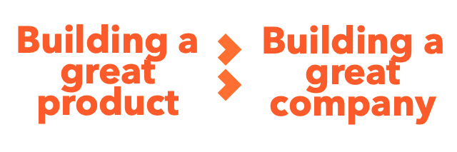
- Great Idea → Great Product → Great Company
- 왜 창업을 하고 싶은가.
- 최고의 이유
- 해당 아이디어는 내가 아니면 안 된다
- 세상이 나를 필요로 한다
- 최고의 이유
- 스타트업을 시작하는 것은 애를 키운다는 것과 비슷하다고 할 수 있다.
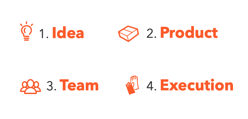
Product : 제품
Idea
좋은 스타트업 아이디어를 떠올리는 방법은 한걸음 뒤로 물러서서 보는 것.
- 의식적이 아닌, 무의식적으로 떠올릴 수 있어야 한다.
- 중요한 것들을 열심히 배우라
- 기술을 배워라
- 최신 기술들을 지켜보기
- 흥미로운 것들을 해봐라
- 기업가 정신은 하나의 도메인 전문가가 된다는 것
- (존경하는) 친구들과 같이 해봐라
- 중요한 것들을 열심히 배우라
사용자 & 고객
- 해결해야하는 문제에 대해 정확히 파악해야 한다.
- ‘문제’ 는 한 문장으로 표현할 수 있어야 한다.
- 어떤 산업군에 속하는가, 산업규모는 어떤가?
해당 산업에 대해서 구체적으로 살펴볼 수 있어야 한다. (2~3 개월) - 제품을 만들 때 모든 관점에서 고객의 입장이 되어보야아 한다.
- 해당 산업의 전문가가 되어야 한다.
- 목표 고객군을 설정해야 한다.
- 코드 작성 전에 사용자 경험을 고려한 스토리보드 작성

- 소수의 사용자가 좋아하는 것에 집중해야 한다.
- 자연스럽게 유저가 늘어날 것
- 제품 런칭 전에 해야할 일은? 딱 10명에서 100명을 위한 기능을 만들어야 한다.
- 창업자가 직접 고객들을 만나야 한다
- 첫 고객에게 집중하라.
- 새로운 고객은 데이트를 하는 것과 같고,
- 첫 인상이 중요하다. 그 느낌을 계속 가지고 이야기할 것이기 때문
- 첫 번째 상호작용을 할 때, 사람들은 인내심이 훨씬 적다.
- 그렇기 때문에 첫 인상을 잘 만드는 것은 제품에 아주 중요하다.
e.g.) Vimeo, Wufoo, Heroku, Chocolat, hurl, MailChimp 케이스, stripe
- 기존 고객은 결혼한 배우자와 같다.
- 성공적으로 잘 사는 관계는 잘 싸운다. (가장 큰 요소)
- Money – Cost / Billing
- Kids – Users’ Clients
- Sex – Performance
- Time – Roadmap
- Others – Others
- SSD: Support Driven Development
- 고품질의 소프트웨어를 개발하는 방법
- 모든 사람이 고객 지원을 하도록 하는 것 → 개발자와 디자이너 모두에게 피드백이 골고루 돌아갈 수 있다.
- 제품을 만든 사람이 직접하기 때문에 최고의 고객지원을 할 수 있다.
- 대화거부는 최악의 행동이며 스타트업에서 많이 하는 실수 중 하나이다.
- Jared Spool, 팀원들이 고객에게 직접 노출되는 시간의 양과 디자인이 좋아지는 정도가 정확히 비례한다. (고객과 실시간으로 이야기를 해야 한다.)
- 최소 6주에 한번은 그런 시간이 있어야 하고, 그 시간은 2시간 이상이어야 한다.
-
감사편지 보내기 – 팀원들이 겸손하려고 했기 때문에 가능한 일 (팀의 조직력을 높이고 팀이 신경쓰는 일을 하게하는 일종의 의식)
- 제일 돈이 되는 사용자들에게 집중하라 → 그 고객들만 잘 관리하면 나머지는 따라온다.
- 고객을 얻는 방법?
- 시작은 지인, 온라인 커뮤니티, 로컬 커뮤니티, 메일, 언론 등..
- 진짜 고객을 만날 수 있는 곳으로 가야 한다
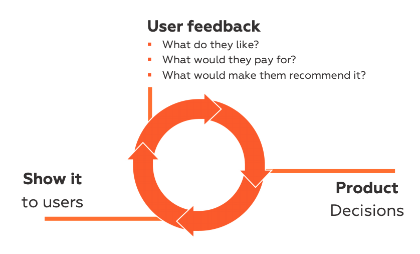
- 고객들에게 피드백을 받아라.
- 피드백이 오는 것보다는 직접 전화를 걸어라, 찾아가라
- 설문: 정말 좋거나, 싫은 경우에만 피드백이 올 것이다.
- 고객의 재방문율을 측정하라.
- 고객에게 돈을 내게 할 수 있다면, 정말 훌륭한 피드백을 받을 수 있을 것이다.
- 더 많은 유저를 위해서는?
- 한가지 초점만 정해놓고, 일주일 내내 집중해야 한다.
- 한 채널씩 이해해야 한다.
- 가장 중요한 부분은 창의력
- 아무도 안 하는 한가지를 찾아서 극단적으로 진행해야 한다.
- 이미 유사한 제품을 사용하고 있는 고객을 끌어오는 방법
- 사용하고 있는 서비스를 전환하는 것은 비용이 든다. 확실한 장점이나 차별성이 있어야 한다. 50가지 자잘한 기능보다는 1, 2 가지의 차별점이 좋다.
Metrics
- Metrics: Focus on growth
- Total Registrations
- Active users
- Activity Levels
- Cohort Retention
- Revenue
- Net Promoter Score
- 이 제품이나 서비스를 동료나 친구들에게 추천할 의향이 얼마나 되시나요?
- Growth : 전환율과 이탈율의 상호작용
- 전환율을 1% 높이는 것과 이탈율을 1% 줄이는 것이 성장에 미치는 영향은 똑같다. 보통은 후자가 더 쉽고 비용도 적게 들어간다.
그 외
- 아이디어, 고객, 산업군에 대해서 알았다면 이제 제품을 만들어야 한다.
- MVP: Minimum Viable Product, 최소생존제품
- 무엇을 하는 제품인지 명확히 정리해야 한다.
(우리 제품은 이런거야 하고 명확하게 말할 수 있어야 한다.)
- 사람들이 좋아하는 제품이란, 해당 제품에 대해서 열광적인 고객층이 있고, 그 고객층이 우리 회사의 제품 뿐아니라 회사 자체도 성공하길 바라는 것.
- 시장을 장악하는 3가지 방법
- 최고의 가격 : 유통
- 최고의 제품 : R&D
- 최고의 종합 솔루션 : 고객 친화
유일하게 누구나 어떤 단계의 기업에서건 쓸 수 있는 방법이다.
QnA 모음
Q. 다양한 고객, 모두가 사랑하는 제품은 어떻게 만들 수 있을까요?
⇒ 초기에는 가장 열성적인 고객에게 집중, 그 고객들에게 맞추다보면 언젠가 일반적인 가치를 발견할 수 있을 것, 기본이 되는 기능들을 만들고 난 후에 그것을 돋보이게 하라
Q. 제품을 만드는 것과 그 외의 일 간의 균형을 맞추는 방법
⇒ 제품에 집중하면서 한쪽에서는 고객과 이야기를 해야하고, 이런 분담은 어느정도 필요하다. 중요한 것은 순환적인 피드백 고리이다.
Q. 제품에 대해 팀 내에서 의견이 서로 다른 경우 의사결정을 진행하는 방법
⇒ 고객 지원을 통해서 해결 (문의가 많은 기능에 대한 기능 순으로 해결)
무조건 고객들이 하라는대로 하는 것이 아닌, 왜 고객들이 그런 요청을 하는지 그 원천적 이유를 찾아서 해결하는 것. 각자의 버전을 만들고 대응해보는 것도 좋다.
Q. Pinterest의 비전이 초창기와 달라졌는가?
⇒ 사람들의 수집품에서 예상하지 못 했던 놀라운 것들을 찾아낼 수 있다는 사실을 나중에 알게 되었다. (사람들의 제품사용 양상이 다른 방향을 보여준다.)
초기에는 누군가 제품을 사용해준 다는 것에 흥분 했다. 재밌는 점은 회사가 성장할수록 포부도 같이 커진다는 점이다. 그래서 항상 Gap이 있다. 우리가 있는 곳과 있어야 할 곳. 객관적으로 우리는 많이 달려왔지만.. 이 Gap은 계속해서 벌어지고 있다.
Execution : 실행
- 실행에 대한 2가지 질문
- 무엇을 할지 정할 수 있는가?
- 그 일을 마무리 할 수 있는가?
- Focus (선택과 집중)
- 가장 중요한 2~3가지 일만 골라서 하는 것
- 커뮤니케이션이 잘 진행 되어야 한다.
- 매주 방향을 공유하고, 디테일한 목표 수치를 향해 달릴 수 있도록.
- 정확한 성과지표를 파악하고, 이 지표가 지속적으로 성장할 수 있도록.
- Intensity (빡세게 일하기)
- 스타트업은 워라밸이 가능한 곳이 아니다.
- 끊임없는 운영 리듬 & 퀄리티에 대한 집착
- 모든 방면에서 빠르게
- Focus (선택과 집중)
- 아무리 큰 일이라도 작은 일으로 나눠서 진행할 수 있다.
- 일을 작은 프로젝트로 나눠서 진행하라.
- 사람에 대해서는 직관에 의존해도 된다.
- 스타트업을 성공시키기 위한 지식은 스타트업을 위한 지식이 아니다.
- 고객에 대한 전문가가 되어야 한다.
- 스타트업에서는 요령피우는 것이 먹히지 않는다.
- 스타트업은 모두 매우 빡세다.
- 스타트업이 성공한다는 것에 대해서는 예측이 불가능하다.
- 운동선수와 수학자처럼 예측이 불가능하다.
- 창업가가 얼마나 강인하고 야망이 있는가.
- 피보팅
- 회사가 성장하지 않을 때
- 제품을 사용자가 사용하지 않을 때
- 논리적으로 비즈니스가 말이 안 될때
- “좋은 계획을 오늘 죽어라 실천하는 것이, 내일에 대한 완벽한 계획을 가진 것보다 낫다.”
- “물건을 부수는 것은 상관 없으니 빨리 움직여라!”
DOORDASH (배달앱) 케이스
- 아무것도 준비되어 있지 않는 상황에서, 바로 랜딩페이지로 서비스 런칭
- 초기에는 아이디어를 시험해보고, 사업을 시작하고, 사람들이 원하는 것인지 확인하는게 중요
- “확장성이 없는 일을 일부로 해라”
- 이 일은 본인의 사업에 있어 전문가가 되게 해준다. 직접 개개인 별로 피드백 메일도 전달.. 등등
- 초기에는 일단 시작을 하고, 제품이 시장에 맞는지 확인해야 한다.
- 정리
- 가설 검증
- 런칭을 빠르게
- 확장성이 없는 일을 한다
수요가 확인 되면 확장을 할 수 있기 때문이다
Teespring (이커머스 플랫폼) 케이스
스타트업이 가지고 있는 가장 원초적인 강점: 확장성 없는 일을 할 수 있는 것
- 첫 고객을 모으고
고객을 모으는 데는 왕도가 없다. 가장 힘든 일일 것이다. 모맨텀을 만들기 까지가 가장 힘들다. 여기서 시간 대비 효율을 따지는 것은 무의미하다. 제품을 무료로 주지 말아라. (제품의 가치를 해치는 일이다., 그래서 지속가능하지 않은 일이 된다.) - 고객을 챔피언으로 만드는 것
입소문을 낼 수 있도록, 기억에 남을 만한 경험을 선사하는 것 (고객과 대화를 하는 방법),
실제 사용자에게 듣는 것보다 제품을 좋게 만드는 방법은 없다.
소셜미디어와 미디어를 확인하라.
중요한 것은 문제를 제대로 고쳐나가는 거이다. (가장 불만이 많던 고객이 가장 영향력이 있는 챔피언이 되어주는 경우가 있다.) - 시장에 맞는 제품을 찾는 것
처음 런칭한 제품은 성장할 수 있는 수준의 제품이 아니어도 된다. 속도가 중요.
경헙으로 얻은 인사이트: 오직 다음 규모의 고객에 대해서만 생각하라
확장성이 없는 일을 최대한 오랜기간 해야 한다.
Growth : 성장
- 성장동력을 유지하는 것 (스타트업 운영의 핵심)
- 항상 이기는 팀을 만들어 내는 것
- 배포에 대한 주기를 정립 (새로운 Features)
- 지표를 공유하는 것
- 매출은 모든 것은 고친다.
- 페이스북 케이스 ‘성장모임’
- 회사의 성장 동력으로 작용
- 지속가능한 성장이 중요하다.
- Sticky :기존 사용자가 계속 방문하게 하는 것
- 좋은 경험이 중요하다.
- CLV (고객주기), Cohort 분석으로 알 수 있다.
- 오랜기간이 지나도 계속 사용하는 고객 → Core 고객들
- Viral : 고객이 직접 주변사람에게 권하는 것
- 좋은 경험이 중요하다. 그것과 함께 입소문을 낼 수 있는 장치가 필요하다.
- 소문을 낼 수 있는 것을 알려준다.
- 제도적인 장치 → 친구를 초대하면 양쪽에 크래딧 제공
- 좋은 경험이 중요하다. 그것과 함께 입소문을 낼 수 있는 장치가 필요하다.
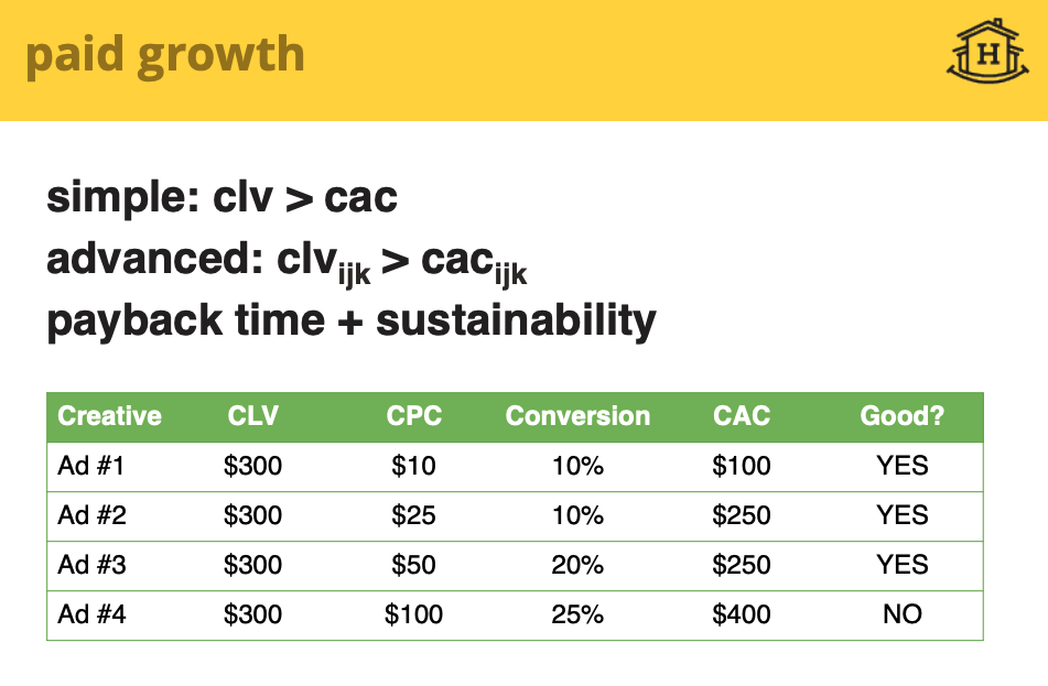
- Paid : 매출을 통해서 돈을 벌고 계속 성장
- CLV > CAC (고객 획득비용) , 돈을 쓰고 더 많은 돈을 얻을 수 있어야 한다.
- 들인 돈을 회수할 수 있는 기간이 중요하다. (3개월 정도)
- Sticky :기존 사용자가 계속 방문하게 하는 것
- 사업할 때 전체 시장크기를 볼 수 있어야 한다.
- 성장에서 가장 중요한 것은 무엇인가?
⇒ 좋은 제품 → 고객 유지 (성장의 핵심) - X축과 평행하게 가면, 시장 크기에 맞는 제품을 잘 만들어낸 것이다.
- Retention이 0 으로 가면 제품이 시장에 맞는지부터 확인을 해야 한다.
- 좋은 Retention 은 몇 프로인가?
⇒ 사업 분야마다 성공을 위한 재방문 수렴치는 다르다. - 스타트업에는 성장팀이라는 것이 있어서는 안 된다. 그 팀 자체가 성장팀을 포함해야 한다.
- 일하는 사람들이 지금 회사에 중요한 것을 알기는 어렵다.
- “마법의 순간”
- 사용자들이 ‘아하’를 경험하는 순간
- 예시)
- 페이스북 → 가입 후 친구의 사진을 보는 순간 (소셜미디어임을 확인하는 순간)
- 왓츠앱 → 친구, 이베이 → 물건 리스트
- 제품의 마법의 순간이 언제인지 생각해보고, 사용자가 그것을 최대한 빨리 느낄 수 있도록 해라
- 성장은 설계하는 것이 아니라 지켜보는 것이다?
- 우리가 초점을 맞춰야하는 고객들은 경계선에 있는 사람들이다. 성장할 때는 이미 잘 사용하고 있는 고객에 신경을 쓸 필요가 없다. 성장에 있어서 가장 중요한 점이다.
- 잘 만들고, 고객을 데려올 수 있어야 한다. (마케팅)
- 유입경로
- Virality : 전파성을 3가지로 나눠 보는 것.
- Payload : 한번의 바이럴 마케팅으로 만들 수 있는 도달의 수
- 전환율(CR) : 전환이 얼마나 일어나는가
- 빈도 : 얼마나 자주 도달 할 수 있는가
- Import → Send → How many People → Click → Sign up → Import …
- K factor로 전파성을 판단
- SEO : 검색엔진
- 키워드 : 어떤 키워드로 경쟁을 할 것인가 정해야 한다.
- PageRank
- Virality : 전파성을 3가지로 나눠 보는 것.
페이스북 케이스
페이스북 성장팀에서 했던 일
- 가입하고 2주 이내 친구 10명을 찾게하는 것
- 국제시장 진출 → 언제든지 확장이 가능한 제품 (느리더라도 제대로)
- 우선 순위의 언어에 먼저 집중
QnA 모음
Q. 이메일 마케팅
⇒ 이메일은 25세 이하는 거의 사용하지 않는다. 메일, 문자, 앱 푸쉬는 동작 방식 전부 비슷, 스팸에 들어가면 안되므로, 우등생? 처럼 메시지를 전달하는 것이 중요하다 중요한 것은 사람들에게 전달이 되어야 하는 것이다.
이 알림은 어떤 경로를 통해 보낼 것인가가 중요하고, 그 다음은 참여를 독려하는 내용에 신경써라.
Business : 비즈니스
- 항상 독점을 목표로 하고 경쟁은 피해야 한다.
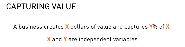
- 사업을 가치있게 만드는 것은 무엇인가?
⇒ X 만큼 가치를 창출하고, Y 만큼 그 안에서 이득을 얻는다. (X, Y는 독립 변수) - 세상에는 ‘완전경쟁시장’과 ‘독접사업’ 두 가지 뿐이다.
- 보통 독점기업은 규제를 피하기 위해서 거짓말을 하고 있고, 완전경쟁시장에서는 1등을 하고 있다고 말하기 위해 독점인 것처럼 말을 한다.
- 교집합 시장이 진짜인지, 말이 되는지, 가치가 있는지 항상 따져보아야 한다.
- 어떻게 독점시점을 만들어 낼 것인가?
- 작은 시장을 노려라. 그 후 그 시장을 구심점으로 확장해라.
- 아주 작은 시장들은 저평가가 되어 있다.
- 작은 시장을 노려라. 그 후 그 시장을 구심점으로 확장해라.
- 독점 기업의 특성
- 자신만의 기술을 가지고 있다.
- 불행한 회사는 닮았으며, 행복한 회사는 각각 다르다.
- 핵심적인 부분에 대해서 혁신적인 개선점을 가지고 있어야 한다.
- 소프트웨어는 한계비용이 0 이다!
- 고정비용은 크지만 한계비용이 작아서 규모의 경제를 갖출 수 있는 경우
- 네트워크 효과는 일반적으로 시간이 지나면서 확장되는 것.
- 자신만의 기술을 가지고 있다.
- 그 분야의 마지막 회사가 되어라
- 가치평가에서 가장 중요한 부분은 지속가능성이다.
- 왜 이 사업이 오랜기간 지속될 것인가를 고민해보는 일..!
- 경쟁은 그 분야에 대해서 당신을 발전하게 만든다. 하지만 정말 중요한 것이 무엇인가에 대한 큰 질문을 하지 못 하면 더 큰 것을 잃는다.
QnA 모음
Q. 아이디어가 독점적인 사업이 될지 아닐지 구분하는 방법
⇒ 실제 시장에 집중해야 한다.
위대한 기업은 다른 기업 들과 다르게 한 단계 더 뛰어넙는 진보가 있었다고 본다.
다른 사람 혹은 심지어 고객의 의견까지도 받지 않고 가는 경우도 있다.
Investment : 투자 유치
- 사업을 한 문장으로 설명할 수 있어야 한다.
- 창업가는 결단력이 있어야 한다. 무슨 일을 하건 일이 진행되도록 해라.
- 최대한 돈 없이 가라. (Bootstrap)
- 투자를 안 받고 가는 것도 충분히 가능하다.
- “성공의 비결은 너무 잘해서 다른 사람들이 무시할 수 없게 하는 것”
- 투자보다 실제로 돈을 벌고 있는 것이 더 어렵다.
- 돈과 리스크와의 관계
- 리스크의 양파이론: 긴 목록의 리스크 리스트가 있을 것이고, 투자의 과정은 투자를 통해 이 리스크를 한 단계씩 제거해 나가는 것이다. 마일스톤을 달성해 나갈 때 마다 리스크를 제거하고, 사업을 진행시키는 것.
- 투자자들에게 NDA (비밀 서약서) 를 써달라고 하지 마라.
- 기록을 하라.
- 좋은 회사로 부터 시드펀딩 → 시리즈 A.. 이런 가능성은 계속 올라가게 된다.
- ⇒ 좋은 투자자는 누구인가?
- 투자 시 협상은 어떻게 하는 것이 좋은가?
- 시드펀딩에서 어디까지 지분을 주는 것이 좋은가?
- ⇒ 20~30%, 30 이상은 주주 쪽으로 문제가 될 여지가 있고,.. 지분이 떨어지는 것에 따라서 동기가 떨어지게 되는데.. 틀이 중요하다. 시드에서는 10~15%, … 외부투자자들과의 관계가 복잡해서 투자를 하지 않는 경우도 많다.
- 최고의 투자는?
- ⇒ Google, AirBnB → 3명의 창업자 모두가 비슷하게 훌륭하기 때문
- 모든 회사는 CEO가 있습니다. 회사를 시작하면 여러분만큼 잘하거나 더 나은 공동창업자를 찾아야 한다. 그것만 해내도 성공할 확률이 천문학적으로 늘어난다.
- 마크 주커버그는 혼자서 이끄는 예외적인 케이스이다.
투자자와 이야기하는 법

- 30초 홍보 : 여러분 회사에 대해 처음 소개하는 것
- 3문장이면 충분하다.
- 첫 문장 – 회사가 하는 일을 소개 (직관적으로 소개, 엄마 테스트 추천)
- 다음 문장 – 시장의 크기 (Botton up analysis)
- 마지막 문장 – 성장률 (빠르게 움직이는 회사임을 보여주라)
- 2분 홍보 : 여러분 회사에 관심있는 사람들을 대상으로 함 (10분 30분 혹은 1시간을 준비하는데, 2분이면 충분하다)
- Unique Insight – “아하” 순간, 이 것을 첫 두문장으로 말할 수 있어야 한다.
- How you make money – 사업 모델, 어떻게 돈을 버는지 혹은 벌 것인지 명확하게 이야기하라
- Team – 1. 팀이 이룬 업적을 자랑 (학위나 상장 X), 2. 창업자의 수 + 기간 + 풀타임
- The Big Ask ($$$) – 자금 요청, 진지한 태도로 임해야 한다.
- When to Fundraise
- 투자자들은 성장률 기반으로 투자하고 싶어한다.
- 여러분이 강하면서 약한 단계 – 자금 요청을 할 시기
- 투자자가 갑이 되는 상황으로 가면 안 된다 – “여러분의 자금 없이는 저희는 아무것도 못합니다” 이렇게 하면 안 된다.
- 투자자와 미팅을 잡는 법
- 이상적: 다른 경영자가 여러분 대신에 회사를 소개해주는 것 (신뢰가는 소개)
- 여러가지 일을 동시에 생각하라
- 투자자들과의 미팅 셋팅을 한 주내에 다 진행해야 한다
- 자금 마련 전담 맴버가 있어야 한다
- 미팅이 끝난 후
- 사후 관리
- 투자자들을 면밀히 조사하라
- 끝낼 때를 제대로 알라
- 회사를 세우라! (자금 마련이 목표가 아니다)
QnA 모음
Q. 어떤 팀, 회사에 투자를 하나요?
⇒ 처음 만나고 1분 정도 이야기하는 동안 정리가 된다. 이 사람이 리더인지, 자신의 제품에 대해서 집중하고 있는지 (질문: 사업을 하게 된 계기), 그 다음으로 보는 것이 커뮤니케이션 능력 → 리더쉽과 훌륭한 커뮤니케이션 능력 이 2가지를 갖추고 있어야 한다.
⇒ 일반적인 2가지.
-
VC 투자 활동은 극히 예외적인 경우만 다루는 게임이다.
4000 개 → 200개만 투자 → 그중 15%가 97%의 수입을 가져다 줌 -
강점이 큰 회사에 투자할 것인가, 약점이 없는 회사에 투자할 것인가
체크 리스트 만으로는 그 팀이 가지고 있는 강점을 제대로 파악할 수 없다.
결점이 있는 회사를 제외 시키면 15% 안에 회사에 드는 회사를 얻기 어렵다.
Q. 초기 자본이 많이 필요한 스타트업에 대해서는 어떻게 하는가?
⇒ 양파 리스크이론을 다시 언급하면, 리스크를 없앨 수 있는 더 구체적인 계획이 필요할 것이다.
Q. 안 좋은 투자자는 무엇인가?
⇒ 네트워크가 부족하거나, 도움을 받을 수 있는 것이 없는 경우, 투자자를 고르는 것은 결혼 상대를 고르는 것이나 마찬가지이다. 약 15~20년 동안 서로를 의지하고 기대면서 같이 나아가는 것이기 때문.
한번 창업가는 영원한 창업가이다.
투자자를 만났을 때, 이 사람이 존경할 만 한가, 배울 점이 많은 가를 고려해보아라.
피투자사와의 관계는 신뢰를 기반으로 해야 한다.
VC의 가장 큰 제약사항은 결국 큰 기회비용이다. 한 분야에서의 최고를 투자하려고 한다.
Q. 제품이 없는 팀이 투자를 받을 방법은?
⇒ 팀이 중요하다. 기본적으로도 팀을 보고 투자하기 때문.
Q. 투자철학을 하나의 문장으로 만드는 것이 필요한가?
⇒ 한 문장으로 정리할 수 있을 정도로 명확한 투자철학을 가지고 있어야 한다. (엘레베이터 피치)
Q. 적합한 시장을 찾는 것 vs 시장을 만들어가는 것
⇒ 굉장히 어려운 문제이다. 투자 철학을 검증하는데 있어, 이 방향이 과연 시장의 존재유무를 확인하는 데에 도움이 되는가이다. 여러분은 현존하지 않는 시장이 여러분만이 알고 있는 근거에 따른 역발상 때문에 창조 가능하다는 주장을 명료하게 펼칠 수 있어야 한다.
Culture : 조직, 기업문화
- 창립자들이 하는 일이 회사의 문화다.
- 믿음은 생각이 되고, 생각은 말이 되고, 말은 행동이 되고, 행동은 습관이 되고, 습관은 가치가 되고, 가치는 운명이 된다. – 간디
- 이것들이 왜 중요한가?
⇒ First Principles (의사 결정의 첫 번째 기준), Alignment, Stability (안정감), Trust, Exclusion (하지 말아야할 것은 아는 것이 더 중요하다), Retention - Zappos의, 첫 번째 핵심가치는 서비스에 “와우” 요소를 넣는 것, 또 다른 핵심가치는 겸손
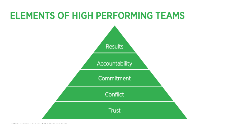
- 성과가 좋은 팀의 특정
- Patrick Lencioni 의 피라미드 – 1. 신뢰, 2. Conflict, 3. Commitment, 4. Accountability, 4. Results
- 인터뷰 과정에서 문화를 고려해야 한다.
- 좋은 문화를 만드는 데 성패가 갈리는 부분은 습관적으로 할 수 있는가 없는가 이다.
- 문화가 일을 해내는 방식이라고 한다면 2가지 요소가 있다.
- 행동양식 (변하는 것), 2. 변하지 않는 것이 필요하다. (핵심가치)
- 여러분만의 핵심가지치 3~4개는 있어야 한다.
- 새로운 사람을 한 명도 고용하기 전에 핵심가치를 정했던 회사! → 첫 번째 개발자를 뽑는데, 걸린 시간은 5~6개월 → 이 사람이 회사의 DNA를 결정하기 때문이다. 다양성은 존중하나, 가치관은 비슷한 사람들이어야 한다.
- 회사의 사명
- ⇒ ‘소속감’을 주고 공통체를 만들어가는 일
- AirBnB의 핵심가치
- 사명을 위해 분투하는 것
- 여기 하는 일에 믿음이 있는가?
- 소명이 있는 사람을 찾는다
- 연쇄 창업가가 되어야 한다는 것 (창조적)
- 사명을 위해 분투하는 것
이것들은 회사의 가치와 원칙으로 변하게 된다.
- 문화의 문제점
- 문화에 대한 글은 찾기 어렵다.
- 정량화하기 어렵다.
- 장기적으로만 효과가 있다.
- 문화는 마치 미래에 투자하는 것과 같다. 결국 장기간 버틸 회사를 만드는데 필요한 것
- 지향점을 확실하게 해야 한다.
- 이 가치들을 기준으로 고용/해고를 해야 한다.
- 여기에 엔지니어가 들어가서 뽑는 것은 좋지 않다. 실력 위주로 보기 때문
- 전반적인 사내문화
- 초기 인력 구성
- 그 이상으로 규모가 커져감에 따라서 발생하는 변화와 적응
QnA 모음
Q. 문화란 무엇일까? → 기업의 문화는 무엇이 되어야 하는가?
⇒ Set of Values?
Q. 기업 문화란 무엇일까?
⇒ 핵심가치, 행동 혹은 행위, 사명감 (목표)
Q. AirBnB 시나이로
⇒ 너무 잘나서 불편하게 할 정도의 팀을 만드는 것이 중요하다. (훌륭한 공동창업자)
제품을 만들고 나면, 회사를 만들어야 한다. → 우리는 오래살 수 있는 회사를 만들고 싶었다. 길게 가는 회사들의 공통점 → 분명한 임무를 가지고 있고, 명확한 가치를 가치며 협업할 수 있다는 것.
Q. 어떻게 집주인들이 AirBnB의 문화를 따르게 할 수 있는가?
⇒ 집주인들은 문화와 맞지 많아도 된다고 생각했지만, 아니였다. (문제가 생기는 등..), 그 이후로는 ‘슈퍼집주인’ 프로그램을 통해서 문화를 따르는 집주인들을 더 대우해준다.
Q. 회사를 만들면서 가장 중요하게 생각했던 요소는?
⇒ 누구를 채용하는가? 채용된 사람들이 무엇을 중시하는지, 우리가 매일 무슨 일을 하는가 또 왜 하는가?, 우리가 소통하기로 선택한 것들, 마지막으로 찬양할 것은 무엇인가?
⇒ 내부 투명성을 더 강조, 모든 직원들이 회사가 하는 바를 지지하고 믿을 수 있도록 하기 위함 (정보를 원활히 접근할 수 있고 상태를 알 수 있다면 도움이 될 것)
⇒ 사내 문화 정립은 다양한 문제를 풀 수 있음, 사람들이 늘어나면서 직접적으로 영향을 끼치는 영향도는 줄어들 수 밖에 없음.
초기에 사람을 10명을 데려오는 것은, 이 사람들이 데려올 90명의 사람들에 대한 영향력까지 고려를 해야하기 때문에 굉장히 조심해야 하는 일이다.
Q. 초기 채용을 하고 올바른 문화를 퍼트리기 위해 한 행동은?
⇒ 언젠가 이루고 싶은 목표를 직원들에게 계속해서 상기시킴, 왜냐하면 누군가에게 문제가 주어지면, 그 사람은 직면한 문제가 세상의 전부라고 생각하게 되기 쉽기 떄문. 많은 시간을 들여서 채용을 한 다음에 입사 후 30일간의 경험을 개선하기 위해 노력한다. (예를 들어, 이름을 아는 동료직원은 있는지? 자신의 매니저가 누군지? 팀원들과 만나고 있는지? 회사에 전반적인 구조는 아는지? 최우선 목표들은 아는지? 이런 프로그램들을 계속해서 발전 시키고 평가함)
⇒ 1. 직원들이 바쁘게 진짜 일을 하는 것. 이렇게 해야만이 실제 문제들을 찾아내고, 얼마나 진척이 됐는지를 알 수 있다. 강하게 적응시키려고 한다. 2. 최대한 빨리 피드백을 주려고 한다. 특히 사내 문화 적응 관련 피드백은 더 빠르게 하려고 한다. (Stripe의 문화 중 하나는 글을 통해서 소통을 하려고 한다.)
Q. Stripe는 어떻게 투명성을 확장시켰는지 궁금하다.
⇒ 스타트업은 정치적인 문제들에 휩싸이지 않은 조직이라고 정의를 했다. 대기업에서는 여러가지 일들이 얽혀있으면서.. 제품에는 최선의 방향이 회사차원에서는 문제가 될 때가 있을 것이다. 하지만 모든 사람들이 한 방향으로 나아가는 스타트업에서는 모든 정보를 공개할 수 있다. Stripe는 초기에 발송되는 모든 이메일에 전직원을 참조시켰다. 일어나는 일들을 미리 알고 있다면, 미팅을 따로 가질 필요가 없다고 생각했다. 하지만 확장에 문제가 있었던 것은 사실이다.
⇒ 첫째는 툴을 바꾼 것이고, 둘째는 확장에 맞춰서 문화를 발전시킨 것이다.
툴은 모든 이메일 공유 → 이제는 매주 취합한 형태로 정보를 공유 (덱을 만들거나..)
문화 이야기는 엄청난 양의 정부가 내부 공개가 되어있고, 이에 따른 사내 규범들이 규정되어 있다.
Team : 동료 & 채용
채용
- 작은 팀으로 얼마나 많은 일을 하는지에 대해 스스로 자랑스러워 해야 한다. 한계에 부딪칠 때까지 초기에는 채용을 하지 않는 방향이 좋다.
- AirBnB 케이스
- 채용 눈높이를 엄청나게 높이고, 천천히 채용하면서 모두가 회사의 일에 대한 사명감을 가지게 함
- 최고의 사람들을 얻는 법
- 똑똑한 사람들은 로켓에 올라타야 한다는 것을 안다. (훌륭햔 제품의 필요성)
- 채용에 사용하는 시간: 0% or 25% (하지 않거나, 최대로 쓰거나)
- 스타트업에서는 중간 실력이면 안 된다. 회사를 망하게 할 수 있다. (이 사람 한명한테 우리 회사의 미래를 맡길 수 있을까?)
- 초기에는 주변 사람들을 영입하는 방식
- 채용시 보는 3가지
- 똑똑한가?
- 일을 해내는가?
- 더 많은 시간을 같이 보내고 싶은가?
- (추천) 인터뷰 보다는 프로젝트를 같이 해보라
- (인터뷰를 할시) 무엇을 해봤는지 프로젝트에 대해서 집중적으로 물어보라
- 레퍼런스 체크를 철저하게 진행하라.
- 그 외 중요한 점들
- 커뮤니케이션 스킬
- 어느정도 위함한 것을 좋아하는 사람
- 스타트업에 대한 집착이 있는 사람
- 마크 주커버그의 기준
- 함께 시간을 보내기 즐거운 사람
- 역할이 뒤집혀도 보고하기 편한사람
- 투자자에게는 협상시 최대를 얻을 수 있도록 하고, 직원에게는 후하게 하라 (지분 등)
- 직원들이 행복하고 존중받는 느낌이 들도록 해야한다.
- 지분 분배의 중요성
- 회사에 일어나는 좋은 일의 공은 모두 팀원들에게 돌리고, 나쁜 일에 대한 모든 책임은 책임을 져야 한다.
- 동기 부여의 핵심
- 자율성 보장
- 성장한다는 느낌
- 일을 하는 명료한 목적
- 해고를 빠르게 해야 한다.
QnA 모음
Q. 초기맴버를 사내문화 관점으로 접근할때 중요하게 본 요소는?
⇒ 같이 일하고 싶으면서 또 재능있는 사람들,
사내문화는 건설한다고 생각하지만.. 내가 보기에는 정원을 가꾸는 일이다.
초기에는 창업자와 비슷한 사람들을 찾으려고 했다. (아주 별난 사람들이기도 함)
우리는 많은 분야에 관심을 가지고 있으면서 한 분야에서는 최고의 전문가인 이런 창의적이고 별난 사람들이 대단한 제품을 만들고 협력에도 뛰어남을 보았다.
우리는 위대한 무언가를 만들고 싶어 하는 사람들이다. 초기 환경을 고려하면 순수한 이유만을 가지고 합류했다.
채용이 이뤄지는 장소, 뛰어난 사람들은 다른 무언가를 하고 있을 확률이 높고 정말 다양한 장소에서 만날 수 있다. 우리는 그런 사람들을 찾아더녀야 한다.
⇒ 신규채용은 장기간 동안 지인의 지인들을 장기간 설득하는 과정이였다.
아직 알려지지 않은, 저평가되고 있는 실력자들
엘레베이터 피치를 하듯, 사람들에게도 이런 과정을 지속해야 한다.
⇒ 첫 10명의 경우, 아주 진실되고 정직했다는 것. 다른 사람들이 같이 일하고 싶은 사람으로서 주변에 믿음을 주고, 문제 접근에 대해 지적으로 솔직한 사람들
특정분야를 파는데 2년을 쏟은 누군가와 일을 하는 것이 당연히 훨씬 더 흥미로운 일, 사소한 디테일이라고 신경을 쓰는 사람들, 그리고 일을 끝마칠 수 있는 사람들
Q. 어떻게 뛰어난 사람을 알아보는 방법은??
⇒ 같이 일해보기 전까지는 100% 확신할 수가 없다.
재능은 2가지 부류로 나뉜다.
- 일을 하는데 필요한 재능들을 미리 알 수 있는 경우
- 그렇지 않은 경우 → 이 경우가 어렵고, 이때에는 누군가와 말하기 전에, 먼저 필요로 하는 분야에서 세계 최고수준이란 무엇을 의미하는지 생각
그 분야에서 세계적인 권위를 가진 사람들과 이야기하면서 그들은 무슨 요소들을 살피는지를 물어보는 것을 습관화하였다. 여기서 무슨 질문을 해야하는지 또한 알 수 있었다.
인터뷰에서의 질문들은 이 사람이 와서 일하기에 적합한가에 대한 답을 줄 수 있어야 한다.
(예를 들어, 문제를 해결하기 좋아하는 사람들에게 구글이 내는 기발한 문제들)
왜 이 아이디어가 좋은 아이디어인지 솔직하게 말하되, 어떤 점들이 어려울지 끔찍할 만큼 디테일들을 늘어놓는 것이 필요하다. (아이폰을 위한 채용 때에는 무슨 일을 하게 될지도 말을 안 했다고 한다. 3년간 가족을 볼 수 없겠지만 일이 끝나면 당신의 아이들의 아이들까지 당신이 만든 걸 기억하게 될 것이다.)
주위 사람들의 평을 받는 것도 중요하다. 경험이 있는 사람들에게 의견을 구하는 것이기 때문. (예를 들어, 인터뷰 때 우리는 모두 조나단을 압니다. 몇주 뒤에 그와 이야기를 하려고 합니다. 그에게 당신이 가장 잘하는 것, 가장 자랑스러워 하는 것, 당신이 나아지려고 하는 부분을 물어본다면 뭐라고 대답했을 것 같나요??)
그 다음에는 가볍게 느껴질 수 있는 질문을 조금 더 게량적으로 느끼게 만들 수 있는 질문을 하고 장기간에 걸쳐 측정을 진행 (예를 들어, 이 사람은 이 부분에서 평가하기에 같이 일했던 사람들 중 상위 1%입니까? 아니면 5%입니까? 아니면 10%입니까?) 상대평가를 강제하면 더 객관적인 평가를 받을 수 있다. 그냥 괜찮다는 말은 도움이 덜 될 수 있다.
⇒ 여러분이 원하는 방식대로 인터뷰를 이끌어 갈 수 있는 자신감이 필요하다. 보통 잘 모르면 알려진 방법들을 따라하게 되는데, 이것보다는 스스로 방법을 알아내는 것이 더 좋은 효과를 준다. (예들 들어, 엔지니어 → 코딩 테스트가 아닌 옆에서 코딩을 하게 하고 그 것을 지켜보는 것, 비즈니스 업무 → 프로젝트 위주로 이야기, 기존 프로젝트를 어떻게 발전시킬지, 어떤 새로운 프로젝트를 하고 싶은지 이야기)
⇒ 첫 10명의 경우, 최대한 일을 많이 해보고 뽑는 것이 필요하다. 모두와 적어도 최소 1주일은 일해보았다. 그리고 한가지 짚고 넘어갈 점은 사람들은 직접 경험하기 전까지는 첫 10명 채용과 사내문화 문제의 중요성을 깨닫지 못한다는 점.
Q. 회사가 10명으로 1000명 규모로 성장함에 따라 채용과 팀관리 정책에 대한 변화는??
⇒ 팀 관리 측면에서는 각각의 팀들이 더 큰 조직에 속한 한계 내에서 최대한 독립적이라고 느끼면서 민첩한 대응이 가능하게 하는 것. 시간에 걸쳐 회사를 여러 스타트업으로 이뤄진 스타트업으로 느끼게 만드는 것. (규격화된 프로세스들 아래 있는 거대한 회사가 아닌..)
한 가지 목표는 각각의 팀이 성과를 이루는데 필요한 자원에 대한 통제권을 가지게 하는 것, 제일 중요한 일이 무엇인지, 어떻게 측정해야 할지 알게 하는 것. 이것들이 이뤄지면 팀 관리가 어느 정도 가능해진다.
각각의 그룹 내에서 해결이 가능하게 하고 싶다. 문제를 어렵게 만들기는 하지만, 이것이 제품을 만드는데 있어 Pinterest가 가지고 있는 철학의 중심가치이다. 여러 분야의 사람들을 모아 놓으면 각자 다른 흥미들을 가지고 있다. 그들을 하나의 프로젝트로 묶고 걸림돌들을 없애주어 마음껏 능력을 펼치게 해주는 것.
채용은 회사 규모가 커짐에 따라서.. 네트워크를 통해서 더 많은 사람을 모을 수 있게 된다. 15 번째 직원이 스타트업과 대기업을 다 경험하면서.. 이런 경험들이 도움이 많이 되었다.
⇒ 변화에 따라서 시간의 길이가 급격하게 변하게 된다. 초기에는 1달 로드맵을 보고 있었다면, 후에는 1년후 나중에는 5년후를 보게 된다. 우리는 미리 계획하고 대비해야 한다.
초기에는 당장의 생산성을 중심으로 사람을 구하게 될 것이다. 그 이후에는 장기적인 관점으로 사람을 채용해야 한다.
시스템을 통해서 문제를 푸는 방법을 고민해야 한다.
Q. 어떻게 사람들에게 스타트업 합류를 하라고 설득할 수 있나요?
⇒ 불확실성이야말로 스타트업이 사람들에게 울림을 줄 수 있는 이유라고 생각한다. 성공이 확실하다면 지루하지 않을까요? 그리고 또 하나의 중요한 동기는 개인 성장 측면이다.
⇒ 무엇이 어려울 것인지, 당신의 최선의 계획은 무엇인지 말해보라. 그리고 그 사람의 역할이 왜 핵심적인지 말해줘라. 반대하는 점은 이 모든 것들을 눈가림 하는 것이다. 예를 들어, 이 문제를 정말 풀고 싶은지 알려면 다른 어떤 회사들에 지원했는지 물어보라. 보통은.. 문제에 집중하는 것이 아니라 괜찮은 회사를 가고 싶은 것이면 유명한 기업들의 리스트가 나올 것이다. 그들은 목적을 이루기 위해서가 아니라 경험을 위해서 합류한 사람들이기 때문이다.
Stripe의 경우는 초기의 4명의 Stripe 사용자들을 채용했다. 다른 방법으로는 구할 수 없었던 인재들이었고, 자신이 좋아하는 제품에서 일하는 것이기에 혜택을 제공했을 것이다.
Q. 사람을 관리하는 방법에 대해서 조금 더 상세하게 알고 싶다.
⇒ 최대 2주에 1번씩은 만나서 1대1 이야기를 해봐라. 토의사항은 매니저가 아니라 직원들이 정할 수 있어야 한다. 정말 신뢰가 쌓였을 경우에는 한달에 1번 정도로 늘릴 수 있을 것이다.
Q. 임원을 해고 또는 강등을 할 때, 어떤 식으로 당사자와 대화하고 어떤 식으로 주변에 설명하는가?
⇒ 누군가를 해고할 때 가장 중요한 것은 솔직해지는 것이다. 감정적이나 감상적은 맞는 방법이 아니다. 채용에서의 실패가 있었다는 것을 인정하고 문제점을 찾아야 한다. (해결의 좋은 시작점)
여러분은 누군가의 직업을 뺐을 수도 있고, 또 그래야만 합니다. 하지만 누군가의 자존심까지 뺏어서는 안 됩니다. (당신의 말이 그 사람의 평판이 될 것, 회사의 문제도 확실하게 인지해야 할 수 있어야 한다.)
Q. 당신에게 반목하던 사람을 자기 편으로 만드는 방법?
⇒ 리더로서 더 나은 방향을 제시할 수 있어야 한다. 말 그대로 당신의 방식이 더 나아야 합니다.
Q. 다른 사람의 입장에서 생각하는 팁
⇒ 일상에서도 어렵지만, 비즈니스에서는 더 어렵다.
아직 절차를 갖춰놓지 않았다면, 잠시 멈춰서 생각을 하세요. 리더가 되기 위한 중요한 자질은 잠시 멈출 줄 알아야한다는 겁니다. 중요한 일이 있는데 아직 생각을 깊이 생각해보지 못 했다면.. 솔직하게 이야기를 해라. “중요한 문제라고 생각하고 다양한 관점을 모두 고려해서 답을 하고 싶다.”
*김치 문제: 작은 감정적인 문제로 숲 전체를 태우는 일 (깊숙히 묻을수록 숙성되는 것??)
Founder: CEO & 공동창업자

- CEO의 일
- 비전 수립
- 투자 유치
- 전도?
- 채용 & 관리
- 실행에 대한 기준을 세우는 것
- 실상 창업자는 사방팔방에서 나오는 문제를 떠안는 사람
- 내가 위대한 창업가인지 어떻게 알 수 있을까?
- 팀
- 혼자서 창업보다는, 2~3인의 공동창업이 낫다 (굉장히 다양한 능력이 요구되는데, 2~3명이 더 다양하게 대응을 할 수 있다)
- 신뢰의 중요성
- 위치
- 위대한 창업자는 반드시 문제와 과업을 해결해 줄 인적 네트워크를 찾기 때문
- 실리콘밸리가 모든 산업에 적합한 곳은 아니다
- 위대한 창업자는 반드시 문제와 과업을 해결해 줄 인적 네트워크를 찾기 때문
- 역발상
- 똑똑한 사람이 이것을 보고 똘끼가 있다고 생각할까? 를 기준으로 삼으면 좋다.
-
- 왜 똑똑한 사람들이 나의 의견에 동의하지 않는가 도 고려해야 한다
-
- 내가 알지만 다른 사람들이 모르는 것은 무엇인가
-
- 똑똑한 사람이 이것을 보고 똘끼가 있다고 생각할까? 를 기준으로 삼으면 좋다.
- 일을 직접 vs 위임
- 간단하게 둘다 해야 한다. (상황에 따라)
- 유연 vs 지속성 (Persistent)
- 역시 둘다 상황에 따라
- 기업처럼 투자철학이 있어야 한다. 그래야 이 기준에 따라서 선택을 할 수 있을 것이다.
- 자신감 vs 주의
- 신념을 고수함과 동시에 다른 사람들의 반론도 받을 수 있어야 한다.
(자신감을 유지하되 위험요소를 충분히 이해하라)
- 신념을 고수함과 동시에 다른 사람들의 반론도 받을 수 있어야 한다.
- 내성적 vs 외향적
- 역시 둘다, 위대한 창업자는 이 경계를 자유롭게 넘나들 수 있다.
- Vision vs Data
- 데이터 역시 당신이 설계하는 비전 안에서 의미가 있는 것이다.
- Data 가 방향을 틀 수 있지만, 명확한 비전은 필요하다.
- Take Risks vs 위험 최소화
- 사업가는 언제나 위험을 계산하고 과감하게 배팅할 수 있어야 한다.
- 위험을 감수할 때, 지능적인 위험 감소를 추구해야 한다.
- 위험은 최소화하되, 효과는 최대화할 수 있는 방안을 항상 강구해야 한다.
- Short Term vs Long Term
- 당연하게도, 둘다 고려해야 한다.
- 팀
- 사업은 절벽에서 일단 뛰어내린 다음, 비행기를 만들어서 나르는 것이다.
- 공동창업자
- 스타트업이 망하는 가장 큰 망하는 이유로 공동창업자 간의 갈등
- 오래알지 못하거나 단순하게 공동창업자를 구하는 것은 재앙이다
- 대학에서 만나면 좋지만, 그러지 못한 경우 회사에서 좋은 사람들 확보
- 오래알던 사람과 창업하는 것이 최선
- ‘거침없는 지략가형’
- 한 분야의 전문가 보다는 007 제임스 본드 같은 사람
- 거칠지만 차분한 사람
- 약 2~3 명이 이상적
- Q. 공동창업자 간의 지분 분배
⇒ 일을 시작한지 얼마 안되었을 때 정리해야 한다. 서로 비슷한 것이 이상적 - Q. 공동창업자 간의 관계가 깨질 경우?
⇒ 이에 대한 안정 장치가 필요하다 (조건부 지분분배)
Management: 경영
- 회사를 설립하는 것은 제품을 잘 만드는 것만큼 어렵다. 기본적으로 사람은 비이성적이기 때문.
- 회사를 설립하는 것은 “엔진”을 만드는 것과 같다. 아주 고성능의 문제가 없을 그런 기계를 만들 수 있어야 한다.
- 매니저의 아웃풋 = 조직의 생산량 극대화 + 주변 팀의 영향력
- 문제에 대한 분류가 필요하다.
감기의 경우, 시간이 지나면 자연스럽게 나아지는 병이므로, 노력을 많이 투자할 필요가 없다. - Editing, 편집자가 창업자에 가장 적합하다.
- 모든 팀원들을 위해 업무를 “명확하게”하고 “단순화”하는 일
- 단순화를 시킨만큼 생산성이 올라갈 것이다.
- 명확하게 만들기 위한 질문을 던져라.
- 자원을 분배하라.
- 여러분과 일하는 사람들 대부분이 자기 고유의 계회을 제시해야 한다. (Bottom-up)
- 빨간 잉크의 양을 체크하라.
-
조직의 일관된 목소리를 유지하라.
- Economist, 글을 보면 한 사람이 쓴 것처럼 느껴질 것이다.
- 위임하기
- 위임의 문제는 결국 여러분(창업자)가 모든 일에 대한 책임을 진다는 점
- 위임과 책임을 동시에 잡는 법
- 과업 숙련도 (task-relevant maturity) 일을 많이 해본 사람에게 더 위임을 하는..
- 경영자는 하나의 관리 방식만을 고수해서는 안 된다. 직원들에게 각가 맞는 방식을 사용해야 한다.
- 결정에 대한 자신감 x 예상되는 결과 영향력 (2 x 2)
- 확신이 적고, 영향력 또한 적다면 완벽하게 위임하라.
- 확신이 크고, 영향이 큰 일은 직접 제대로 하라.
- 과업 숙련도 (task-relevant maturity) 일을 많이 해본 사람에게 더 위임을 하는..
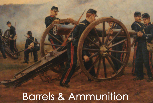
- 팀을 구성하기
- 포와 탄약에 대한 비유, 채용되는 사람들은 대부분 탄약이고 그것을 움직이는 대포와 같은 소수의 사람들이 있다.
한 번에 쏠 수 있는 탄약의 수는 대포의 수에 의해서 결정된다.
대포같은 사람이란, 특정 아이디어를 구상단계에서부터 실제 상품을 고객에게 전달하고 사람들을 결집시킬 수 있는 사람이다. 문화적인 기량이 상당히 필요하다. - 대포를 늘리기 위해서는, 모두에게 결국 부러질때까지 점진적으로 책임의 볌위를 늘려나가는 것이 필요하다. 실패의 시점을 기억하고 그 수준으로 책임을 부여하면 된다.
- 수평적인 관계에서 주변 동료들이 많이 찾는 사람이 있다면, 그 사람은 주변 사람들을 도와주는 사람일 것이다. 즉, 대포에 가까운 사람일 것이다.
- 포와 탄약에 대한 비유, 채용되는 사람들은 대부분 탄약이고 그것을 움직이는 대포와 같은 소수의 사람들이 있다.
- Scaling, 언제 어떻게 확장을 할 것인가
- 각각 회사마다 성장곡선이 다르다.
- Insist on Focus, 한 가지 일에만 집중하게 하는 것
- Peter 의 방식, 사람은 눈에 보이는 쉽게 해결할 수 있는 일을 먼저 처리하기 때문 → 누구도 문제를 제대로 풀기 위해서 시간의 100%을 사용하지 않는다.
- Metrics & Transparency
- Dashboard를 만들기를 추천한다.
- 첫 대쉬보드는 창립자가 만들어라.
- 이 대쉬보드에는 무엇이 중요한지 모두가 알 수 있도록 직관적이고 명확해야 한다.
- 투명성
- 회사의 모든 직원들은 회사내 벌어지는 모든 일을 알 수 있어야 한다.
- 이사회의 결정이 나는 발표자료를 모든 직원들에게 공유
- 모든 미팅에 대해서 전체 공유
- 회의실 벽이 모두 유리로 되어있다.
- 스티브잡스 Next → 투명 임금제도
- Metrics
- 한가지 요소에만 집중하지 말고, 트레이드오프가 되는 요소까지 같이 측정해야 한다. + 책임을 지는 사람의 수준
- Dashboard를 만들기를 추천한다.
- 예측이 불가능한 현상에 대한 분석이 필요하다. → 새로운 시장을 개척할 수 있는 기회
- Details Matter
- “모든 디테일을 잡는다면 100만달러짜리 사업을 시작하거나 100만불의 수익을 창출하거나 100만명의 사용자를 잡기위해 노력할 필요가 없다.”
- 조직전체가 모든 일을 제대로 한다면, 결국 최고 수준의 팀을 가지게 될 것이다.
- 직원들이 매일같이 일하고 살다시피하는 사무실 환경은 기업의 문화와 사람들이 결정하는 방식과 직원들이 투입하는 노력의 정도를 결정할 것이다. 이러한 디테일을 다른 사람에게 맡기지 말고 스스로 해라.
- One Management Concept : 결정적인 결정을 할 때는, 그 결정에 대해서 바라보는 모든 사람들의 시각을 이해할 필요가 있다. 즉, 회사 전체의 시각에서 문제를 바라볼 수 있어야 한다.
- Demotions
- 해고 vs 강등
- 해고보다는 강등을 포함한 옵션을 주는 것이 개인에게도, 결정권자 입장에서도, 회사입장에서도 더 나을 것이다.
- 강등 후, 사람들의 신임을 얻을 수 있을 것인가 또 당사자가 동기부여를 잃어버리지는 않을까
- 이것은 고소득을 올리는 직책의 직원이 자신의 임무를 다하지 못했을 때 일어날 수 있는 일을 정의한다.
- 해고 vs 강등
- Raises
- 우수한 직원이 임금 인상을 요구한 경우
- 직원 입장에서는 이러한 요구를 하기까지 굉장히 많은 단계를 거쳤을 것
- 임금 인상을 요구하지 않는 직원들도 고려를 해야 한다.
- 절차(원칙)는 중요하다. → 사내 문화를 보호할 수 있는 수단
- 우수한 직원이 임금 인상을 요구한 경우
- Sam Altman blog post
- 스톡옵션을 행사하는 방법에 대한 제안 (행사가능 기간 10년)
- 현재: 퇴사 후 90일 내에 처리를 해야하는 상황 + 행사를 하려면 필요한 돈의 문제
- 90일로 선정이 된 이유는 주가에 대한 불확실성으로 손실 계산이 불가능했기 때문이다.
- Cultural Statements (2가지의 대안책들)
- 직원들에게 솔직해지기, 10년후에도 행사할 수 있는 조건
- 사실 그대로 말해주기, 스톡옵션이라는 권리가 주어질 것이나 회사에 남아있어서 상장까지 시킬 수 있어야 받을 수 있는 권리다 → 어떤 사람을 채용하고 싶은지 말하는 바가 있다.
- 스톡옵션을 행사하는 방법에 대한 제안 (행사가능 기간 10년)
- History’s greatest practioner
- Toussant (투싼) 에제
- 주변의 적과 싸워서 이겨야 했다
- 자국의 군대 입장
- 적의 입장
- 나라의 문화 입장
- ⇒ 약탈을 하지 않음, 강간 X, 장교 간의 불륜 X (장기적인 문화를 고려했기 때문)
- ⇒ 전쟁에서 이겼을 때, 적군의 능력이 있는 장수를 고용 (전문성과 더 높은 수준의 문화를 원했기 때문)
- 노예주에 대한 처분
- 노예들의 입장 (노예주를 죽이자)
- 투생의 입장 (기존의 노예로서의 입장, 설탕경제에 대한 이해)
- 노예주들의 입장 (사업을 하는 방식)
- ⇒ 노예제 폐지, 노예주는 땅을 그대로 소유하되 임금을 지불, 강제 노동 금지 (마찬가지로 더 높은 수준의 문화를 원했기 때문)
- 주변의 적과 싸워서 이겨야 했다
- Toussant (투싼) 에제
- Demotions
결론 : 여러분이 배울 수 있는 가장 중요한 일이자 CEO 로서 가장 어려운 일이 바로 스스로가 회사를 직원들과 파트너들과 관점에서 바라보도록 훈련시키는 일이다. 여러분과 이야기하고 있지 않고 한 공간에 있지 않은 사람들의 관점에서 말입니다.
QnA 모음
Q. 탄약을 언제 많이 뽑아야 하나요?
⇒ 엔지니어의 경우에는 10~20명 정도가 충분할 것 같고, 포가 준비되었을 때 탄약을 뽑는 것이 맞다고 본다. 디자이너의 경우에는 조금 다르다.
X (총 생산량) / Y (팀원의 수) → 이 값을 가지고 직무평가를 한다고 해야 한다.
이럴 경우 Y 는 늘어나지 않을 것이다.
Q. 위임과 책임 그리고 디테일에 대한 조화를 어떻게 이룰 것인가?
⇒ 디테일을 잡는 다는 철학은 기업 초기에 매우 중요하다. 기준을 잡는 일이 때문.
그래야 나중에 들어온 사람들도 이 기준에 맞춰서 일을 할 수 있게 될 것이다. 문화는 곧 결정을 내리게 하는 사고의 틀이다.
User Interview: 사용자 인터뷰
- Emmett – Twitch CEO
- 누구와 대화를 하는지, 또 무엇을 묻고 얻을지는 굉장히 중요하다.
Twitch의 경우, 시청자와 방송제작자의 피드백은 완전히 다를 것이다. - 강의 중심의 노트 필기 앱 케이스
- 여러분이 만드는 것에 대해서 배우기 위해서는 누구와 말을 해야 할까요?
- 예시
- 실제 강의를 듣는 학생들
- 학원을 안 가고 집에서 인강을 듣는 사람들
- 각각 다른 과목을 듣는 사람들
- 공부 방법 별로 분류해서 만난다
- ⇒ 학생들은 돈을 잘 쓰지 않는다. 오히려 대학 IT 서비스 팀 혹은 부모들을 대상으로 판매를 계획하는 것이 더 맞는 방향일 수 있다.
- 강의를 하는 선생/강사
- 영상으로 편집하는 편집자
- 실제 강의를 듣는 학생들
- 뭔가 대단한 아이디어가 있다면, 생각할 수 있는 가장 넓은 그룹의 사용자들을 생각해보라.
- 예시
- 인터뷰를 통해서 무엇을 만들지 정해보자.
- 질문에 꼬리에 꼬리를 물면서 더 세부적으로, 파고든다.
- 첫 인터뷰에서는 기능에서 최대한 멀어져서, 문제에만 집중을 해야 한다.
- 다양한 사람들과 문제에 대해서 이야기를 하다보면 큰 장애물이 있는 부분을 알게 된다. 이 부분이 제품의 핵심이 될 수 있다.
- 한 분야의 6~8명을 인터뷰하면 정보를 거의 얻었다고 볼 수 있다.
- 인터뷰를 바탕으로 기능을 생각해보자.
- 이 기능이면 충분한가? 이것을 보고 사람들이 우리의 제품으로 전환을 할까요?
- 직접 프로그래밍을 해서 세상에 공개한다.
- 위의 방법은 시간이 걸리기 때문에, 프로토타입 기법을 활용한다.
- 이때, “내가 이런 기능을 생각해봤어” 라는 식으로 접근하면 좋은 피드백을 얻을 수 없다.
- 기능을 평가하기 위해 최소한으로 가져야 하는 방법으로.. 다른 제품에 붙여보고, 사람들이 사용하는지 확인해보는 것
- Money Test는 실제로 사람들이 돈을 주고 이 제품을 살 것인지 말해준다.
- 이 기능이면 충분한가? 이것을 보고 사람들이 우리의 제품으로 전환을 할까요?
- 여러분이 만드는 것에 대해서 배우기 위해서는 누구와 말을 해야 할까요?
- Twitch 케이스
- 몇 가지 피드백을 보면.. 이런 이슈들이 있음에도 해당 제품을 사용한다는 것은 굉장한 의미가 있다.
- 다른 제품 유저들의 피드백을 보면 완전히 다른 양상의 피드백을 얻을 수 있다.
- 방송제작자의 피드백, 경쟁제품을 사용하는 방송제작자의 피드백, 일반 사용자의 피드백
- 게이밍 방송시장의 경우, 일반사용자가 대부분이고 더 큰 시장임을 의미한다.
- 유저 인터뷰를 한 사람들을 대상으로 문제점을 파악하고, 제품을 만들어서 제안!
- 데이터를 기반으로 판단하는 것은 좋으나, 제품의 방향을 보여주지는 못 한다.
QnA 모음
Q. 스타트업이 인터뷰를 할때 실수하는 것들은?
⇒ 제품을 보여주지 말라. 제품을 보여주는 것은 기능에 대해서 말해주는 것과 같다.
사람들의 머리속에 있는 것을 파악해야지, 새로운 것을 넣으면 안 된다.
실제로 인터뷰해야 하는 사람이 아닌 대화 가능한 사람을 하는 경우가 많다. 실제 사용자가 누구인지 알아내는 과정이 필요하다.
Q. 회사 내 다른 사람들을 설득하는 방법
⇒ 인터뷰를 녹음해라. 만약 여러분이 어떤 것을 만들어야 된다고 주장하고 싶으면, 그저 인터뷰를 재생해주면 된다.
Q. 인터뷰를 어떤 툴을 통해서 진행했는가?
⇒ 이메일보다는 Skype와 같은 툴에서 진행해야 한다. 가장 흥미로운 포인트들은 “흥미롭군요, 좀 더 말씀해주세요” 에서 옵니다. 의도하지 않았던 순간에서 핵심이 나온다. (상호적인 피드백이 중요한 이유)
Q. 글로벌 시장에서의 인터뷰는 (다른 언어의 사용자들)?
⇒ 한국 시장의 경우, 통역자를 구해서 인터뷰를 해봤으나 실제 사용자의 대표를 구하기 어려운 문제가 있다.
Q. 인터뷰 대상자를 구하기 위한 채널과 보상은?
⇒ Twitch의 경우, 회사 웹사이트 내의 메시지 시스템이였다. (채널), 돈을 지불하면서 대화를 할 필요는 없었다. 보통 문제를 직시하고 있는 사람들은 보상없이 자신이 원하는 바를 이이기 한다.
Q. 사이트 자체적인 유저 피드백 도구들이 있나요?
⇒ 중요한 두번째 종류의 유저 피드백이 있다. 우리는 문제를 발견하는 것에 집중했기 때문에 사이트가 없었다.
Q. 제한된 리소스 상황에서 하나의 고객군에 집중해야 한다면?
⇒ 우리는 경쟁 제품을 사용하는 사람들에게 집중했다. 이미 우리가 요구하는 행동에 관심이 있었고, 이런 요구를 만족하면 옮길 것이라고 생각했기 때문이다. 또 회사 상황상 빠른 성장을 해야하는 상황이였다.
Q. 게임 퍼블리셔는 어떻게 대하였는가?
⇒ 누구도 대화를 하려고 하지 않았다. 제품을 사용자들이 많이 쓰게되면서 자연스럽게 퍼블리셔에게 우리가 중요해졌고, 대화를 하게 되었다.
제품은 계속해서 변화하고 그 때에 맞는 사람들과 대화를 하는 것이 중요하다.
Q. 사용자 입장에서 좋은 피드백을 주는 방법
⇒ 생각하는 진짜 문제를 이야기해줬으면 좋겠다. 횡성수설 했으면 좋겠고.. 그냥 아무 말이나 해줬으면 좋겠다. 그 사람에 대한 컨텍스트를 알 수록 무엇을 원하는지 알 수가 있다.
Legal & Accounting: 재무기초
- 자금 마련, 직원 고용, 계약 체결
- Delaware Corporation (델라웨어 회사법)
- 내가 이 일을 개인으로써 하고 있는지, 독립된 법인체인 기업을 대신하여 하고 있는 것인지
- 자본 배분
- 지분
- 공동창업자들간의 지분관계 → 모든 창업자들이 동등한 배분을 받았다
- 과거가 아닌 미래에만 집중
- 주식 배분
- 83(b) Election
- 서류에 서명하고 그 증서를 가지고 있어라
- 주식의 귀속 (Vesting)
- 실리콘밸리 표준 4년, 클리프 1년: 1년 후 25%를 가지고, 점진적으로 가짐
- 이 제도를 사용하는 이유? → 창업자가 퇴사를 하는 경우, 오랫동안 일할 수 있는 동기부여의 필요
- Fundaraising
- 벨류에이션 캡
- 예) 500만 달러 캡, 10만 달러 투자 → 회사의 가치가 2천만 달러, 한주당 25센트로 구입 가능
- 미래에 주식이 희석될 수 있음을 알려라
- Investor Requests
- 이사직 : 왠만하면 거절하는 것이 좋다, 전략과 방향성을 제시해줄 수 있는 인재는 돈으로도 살 수 없다
- 어드바이저: 도움이 되는 조언을 하는 경우가 드물다, 투자를 한 이상 도와주는 것은 당연한 일이다.
- pro-rata 권리: 미래에 추가적인 주식을 매입함으로써, 회사 내의 지분을 유지할 수 있는 권리
- 정보에 대한 권리: YC는 한달에 한번씩 투자자들에게 업데이트를 추천
- Company Expenses
- 사무실 대여, 직원 고용 등등
- “내가 각 세부 사항을 이야기해야할 때, 부끄러울 항목이 하나라도 있는가?”
- 각종 영수증은 챙겨야 한다
- 창업자 고용
- 창업자가 무급으로 일하는 것은 불법이다.
- Payroll Service를 사용하라
- 창업자가 퇴사하는 경우, 문제가 되는 경우가 존재
- 직원 고용
- 정규직과 계약직의 차이
- 근로자 관련 보험, …
- 이 역시, 스스로 업무를 보는 것보다는 서비스를 이용하라
- 직원 해고
- 가능한 빨리, 명확하게 진행하라
- Legitimacy
Sales and Marketing: 영업과 마케팅
- 영업 → 창업을 하면 창업자가 하게 될 것
- 제품, 산업 도메인에 대한 이해필요

- Almighty Funnel – 1. Prospecting, 2. Conversations 3. Closing 4. Revenue / Promised Land
- 각 단계별로 효과적이였던 전략
- Prospecting
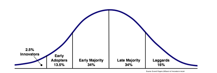
- 기술 수용 주기
- 얼리어답터 = 잠재적 고객 (약 2.5%)
- 이 말은 곧 약 2.5%의 고객들만이 전화를 받고 고민할 것이라는 것
- Top 3: Your network, conferences, cold emails
- 컨퍼런스: 초기 고객들을 만날 수 있는 장소,
- 기술 수용 주기
- Conversations
- 전화를 받으면 그들이 말을 하게 하라!
- 영업의 1%의 사람의 경우, 70%는 그들이 이야기하게 하고 30%정도를 이야기 한다. 특히 문제를 제대로 이해하기 위한 질문을 한다
- 통화 후 사후관리
- 이메일(응답 없음) → 이메일 x n
- 시간은 스타트업의 자산이다 → 초기에 살만한 고객인지 아닌지를 빠르게 구별할 수 있어야 한다.
- 전화를 받으면 그들이 말을 하게 하라!
- Closing
- 표준 계약 서식
- 사소한 부분에 집착하면서 시간을 잃지 말라.
- “제품은 마음에 드는데, 이 기능이 있으면 좋겠네요” → 기능을 추가해도 이 사람이 쓴다는 보장은 없다.
- 해당 기능을 추가하는 것으로 계약을 체결
- 다른 고객들의 이야기를 종합하여 기능 추가를 판단
- Free Trials: 프리 트라이얼 이후에 구매를 요구하는 것은 다시 제품을 파는 것이나 마찬가지이다. 누군가 프리 트라이얼을 요구한다면, “저희는 주로 연간 단위로 계약하는데, 이번에만 처음 30일, 60일 이내에 제품이 마음에 들지 않으시면 취소하실 수 있습니다”
- Revenue / Promised Land
- 5가지 비즈니스방법 – 자신의 사업이 어디에 속하는지 확인하라
- 10$, 10,000k Customer : Marketing
- 100$, 1,000k Customer : Marketing
- 1,000$, 100k Customer : Marketing
- 10,000$, 10k Customer : Inside Sales
- 100,000$, 1k Customer : Field Sales
- 5가지 비즈니스방법 – 자신의 사업이 어디에 속하는지 확인하라
- Prospecting
B2B: 기업용 소프트웨어
- Aaron Levie, Box CEO
- 항상 변화하는 기술적인 요소를 주목하라.
- Box – 파일 공유에 집중,
소비자들에게는 더 많은 기능을 제공하고, 기업용으로는 보안 등.. 요구사항을 충족하지는 못하고 있던 상황 - 소비자 / 기업 간의 시장 규모 → 가치에 대한 등식이 다르다
(소비자 돈을 최대한 적게 쓰려고 하고, 기업 입장에서는 돈보다는 효율과 효과에 집중) - On-Premise ↔ Cloud
2명~ 30만명까지 다양한 기업을 지원할 수 있다는 것은, 진입할 수 있는 시장이 확대되는 것을 의미한다. - 기업에서 기술 혁신이 일어날 때, 딱 2번의 기회가 있을 것
- 원자재가 변화할 때 → 컴퓨팅 가격이 낮아지는 등
- 고객들이 기업의 제품에 대해서 새로운 경험을 필요로 할때 → 운송업에서의 우버
⇒ 지금이 단 하나의 산업군을 타겟으로 하는 수직적 소프트웨어 회사를 시작하기에 좋은 시간인지 보여준다. → 모든 분야에 적용할 수 있기 때문
- 앞으로도 회사들은 더 똑똑하고, 효율적으로, 효과적으로 일하기 위해 나아갈 것이다.
- 창업 관점에서의 조언들
- 기술의 변화를 찾아라. – 크고 근본적인 트렌드의 변화
- 잘 살펴보면, 지금 적용되는 기술들은 이미 몇년 전에 시도했던 기술들일 것이다. (환경이 받춰주지 못했기 때문에)
- 의도적으로 작게 시작할 필요가 있다. – 이미 존재하는 제품들 사이에 끼어들 수 있는 쐐기 같은 제품이어야 한다.
- 불균형을 찾아야 한다. – 기존 업체들이 하지 못했거나, 하지 않은 일을 해야 한다.
- 아웃라이어를 찾아야 한다. – 제품의 얼리어답터를 활용하라.
- 고객의 말을 들어가 – 하지만 항상 이들이 원하는대로 해주지는 마라. 요구사항을 듣고 해석해서 정말 좋은 것을 만들 수 있어야 한다.
- 커스터마이징이 아닌, 모듈화를 해라
- 사용자에 집중하라 – 기업용 소프트웨어에 소비자 DNA을 넣어라.
- 바이럴 마케팅이 가능하게 하라. – 근본적으로는 제품이 중심에 있어야 한다.
- 기술의 변화를 찾아라. – 크고 근본적인 트렌드의 변화
Later-Stage Adivce: 후기 단계의 조언들
- 창업 후 12~24개월 후에 중요해지는 일들
Management
- 약 25명의 직원이 있는 다음, 갑자기 구조의 부재를 느끼는 순간이 올 것
- 해야할 것은 모든 직원들이 그들의 관리자가 누구인지 알게 하고, 직원마다 관리자가 한명이도록 하는 것. 마지막으로 모든 관리자들은 직접 보고해야할 대상을 아는 것.
- 명확한 보고 체계가 중요
- 관리구조를 혁신하려고 하지 마라. 혁신해야 할 것은 제품이다.
-
훌륭한 제품을 만드는 것에서 훌륭한 회사를 만드는 일로 변경 된다.
- 실패케이스
- 경력자 (시니어) 채용을 주저하는 것
- 영웅모드 (본보기)
- 나는 휴가를 쓸 것이고, 직원을 더 뽑을 것이야. 앞으로 성장을 이 만큼 할 것이니 그것에 맞춰서 고용을 할 것이다.
- 나쁜 위임법
- 나쁜 케이스 : 우리는 큰 일을 해야한다. 이것을 조사해주세요. 그럼 제가 결정하고 진행하면 됩니다.
- 좋은 케이스: 우리는 큰 일을 해야 한다. 나는 당신을 신뢰하고 있다. 조사하고 어떻게 결정할지 알려주세요.
- 개인적인 정리
- 개인의 생산성과 제품의 개발을 추적하는 일은 꼭 필요하다.
- 추가로 단순히 어떤 일을 하고, 왜 그 일을 하는지 써 놓는 것도 중요하다. (‘어떻게’ 와 ‘왜’)
- 이것이 회사의 규범이 될 것이다.
- 왜 → 문화적 가치
HR
- 명확한 구조 : 성과에 대한 피드백이 중요
- 회사가 성장함에 따라서 보상 밴드가 필요해질 수 있다.
- 지분 : 많은 주식을 직원들에게 나눠주라
- 향후 10년간 3~5%를 회사의 직원들에게 나눠주어라
- 개인적인 추천: 6년 Vesting
- 옵션 관리 시스템의 필요성
- 50명 이상의 직원일 때
- 성추행, 다양성에 대한 교육
- 번 아웃이 되지 않도록 관찰하기 → 이제 마라톤이 되기 때문에
- 채용 절차
- 채용하기 전에 내부 내정자를 내부 메일링 등을 통해서 공지
- 직원 늘리기 프로그램
- 팀의 다양성
- 초기 직원들에 대한 관리
- 일반적으로 회사가 직원들보다 빠르게 성장한다
- 직접적으로, 솔직하게 이야기해보라 → “초기 직원들은 회사가 성장함에 따라서 무엇을 하고 싶을까”
Company Productivity
- 초기에는 고려할 사항이 아니다.
- 직원이 늘어나면서 생산성은 직원 수의 제곱으로 떨어진다.
- 중요한 하나의 단어: Alignment
- 모두 같은 페이지에 있고, 하나의 방향을 보게 하는 것
- 방법 중 하나는 명확한 로드맵과 목표를 가지는 것
- 무작위로 직원 중 3명에게 회사의 최상위 목표 3가지가 뭐냐고 물어보면.. 답을 할 수 있어야 한다
- 만약 사람들이 결정의 뼈대(토대)를 알고 있다면, 같은 결정을 내릴 것이다.
- 프로세스가 아닌 제품에 의해서 움직이고, 매일 딜리버리해라.
- 커뮤니케이션 : 투명성과 리듬
- 주간 관리회의
- 매월 로드맵과 비전을 공유하는 올헨즈미팅
- Offsite (워크샵)
- 목표는 오랜 기간 가치를 만들어내는 회사를 만드는 것
- 창업자들이 끌고가면서 하나의 제품에 혁신이 있을 수 있으나, 그 다음 것까지 혁신을 이룰 수 있어야 한다.
Mechanics
- 회계, 재무 등
- FF Stock (Founder’s Fund) in the B round
- 지적재산권, 상표, 특허
- 제품 출시 후, 11개월 후 정도가 적당하다. 임시특허
- 상표권, 도메인 등
- FP&A : 재무 모델
- 세금 구조 짜기
Your Psychology
- 갈수록 더 강도가 강해질 것이다.
- 성공을 하게 된다면, 많은 haters가 생길 것이다. 그것을 무시해라.
- 장기적인 관점을 가지는 것.
- 지독한 번 아웃을 경험할 수 있다.
- Focus
- 인수합병에 관심을 가지지 말라. → 회사를 죽이는 방법이다
- 스타트업은 창업자가 포기할때 망한다
Marketing & PR
- 제품이 팔리기 시작하면, 그떄부터 조금씩 신경을 쓰라
- 핵심 메시지는 창업자 스스로 찾아야 한다. → 회사가 어떤 메시지를 결정하는 일
- 개인적으로 핵심적인 기자와 관계를 만들어라 (대행사를 교용하는 것보다 더 직접적으로 의견을 전달할 수 있다)
Deals
- 좋은 제품을 만드는 것
- 개인적인 관계를 발전 시키는 것
- 경쟁 역학
- 창업자서의 고집은 불편할 정도가 되어야 한다
- 원하는 것이 있으면 요구하라
- 스타트업이 겪는 그래프
QnA 모음
Q. 다양성에 대해서..
⇒ 원하는 것은 배경의 다양성이지, 비전의 다양성이 아니다. 배경의 통일은 획일화된 문화로 이기어지 때문이다.
Q. 개인적인 차원에서 생산성을 끌어올리는 방법
⇒ 3달에서 12달정도 시간 동안 해야하는 목표를 적은 종이를 만드는 것. + 매일보기
별도로 단기 리스트, 모든 사람들에 대한 리스트 (하는 일, 나눈 대화, 그외 정보들)
Q. 스타트업이 잘 실패하는 방법
⇒ 실패하고 있다면, 투자자들에게 말을 하고.. 자금이 바닥나지 않도록 해야한다. 빠르게 행동해야 한다. (직원들에게도, 투자자들에게도)
Q. YC 내 이민자 출신의 창업자 수
⇒ 41% 정도??
Q. 전문적인 CEO를 고용하기에 적절한 시기는?
⇒ Never, 창업자가 계속해서 운영을 하는 것, 좋은 제품을 만드는 관점으로는 꼭 그래야 한다
Q. YC가 스타트업을 선정하는 기준, 그리고 시간이 지나면서 변하는지?
⇒ 좋은 창업자와 좋은 아이디어. 기준은 변하지 않았다.
Q. 좋다고 생각하는 시장이 있지만, 아직 많이 알지 못하는 경우의 접근 방법
⇒ 1) 그냥 바로 들어가는 것, 하면서 배우라.
⇒ 2) 그 분야에 있는 회사에서 일하거나, 그 시장에서 1~2년간 무엇이라도 하는 것
후자를 약간 더 추천한다. 그러나 사용자에 대해 정말 제대로 배울 생각이 있다면 크게 상관 없다
끝으로
이번 기회에 다시 정리를 해보면서 내용들을 여러번 다시 보게되었습니다. 대략 7년이 지난 지금에도 적용이 되는 이야기가 대부분이라고 생각합니다. 각 강의에서 창업자들의 인사이트가 느껴지기도 하구요. 스타트업이 성장하고 커가는 방식은 다양할 수 있지만, ‘훌롱햔 제품을 만드는 것’ 이 가장 기본이 되는 방식일 것입니다.
언젠가는 훌륭한 제품 그리고 훌륭한 회사를 만들고, 위 강의처럼 인사이트를 공유해보고 싶네요.