Seeing is believing: a client-centric specification of database isolation, Crooks et al., PODC’17.
Last week we looked at Elle, which detects isolation anomalies by setting things up so that the inner workings of the database, in the form of the direct serialization graph (DSG), can be externally recovered. Today’s paper choice, ‘Seeing is believing’ also deals with the externally observable effects of a database, in this case the return values of read operations, but instead of doing this in order to detect isolation anomalies, Crooks et al. use this perspective to create new definitions of isolation levels.
It’s one of those ideas, that once it’s pointed out to you seems incredibly obvious (a hallmark of a great idea!). Isolation guarantees are a promise that a database makes to its clients. We should therefore define them in terms of effects visible to clients – as part of the specification of the external interface offered by the database. How the database internally fulfils that contract is of no concern to the client, so long as it does. And yet, until Crooks all the definitions, including Adya’s, have been based on implementation concerns!
In theory defining isolation levels in terms of what the database does on the inside should at least be helpful to database developers – although as we’ll see in actual fact it can be over-constraining – but it leaves the much larger number of database users with a harder task to figure out what that means in terms of the effects visible to their applications.
This paper introduces the first state-based formalization of isolation guarantees. Our approach is premised on a single observation: applications view storage systems as black-boxes that transition through a series of states, a subset of which are observed by applications.
With isolation levels defined in terms of observable states, it becomes immediately clear to application developers what states their applications may observe, and it gives the implementors of storage systems maximum freedom in terms of how they meet the required external guarantees. In case you need any further motivation to dig in, in a panel at the Papers-we-love mini-conference earlier this month, this paper was nominated by Joe Hellerstein as a hidden gem deserving of wide visibility.
A motivating example
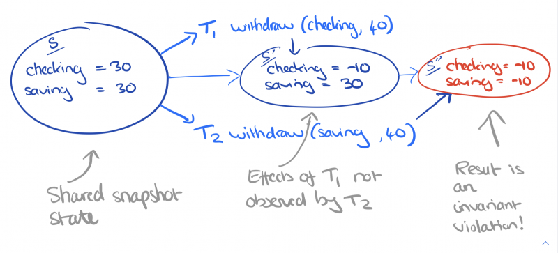
I’m going to jump ahead in the paper and start with a motivating example. Alice and Bob are joint owners of linked checking and savings accounts at a bank. The bank allows withdrawals from either account, so long as the combined balance remains positive. A withdrawal transaction is given an account and an amount, checks that the combined balance is sufficient to cover the withdrawal, and then debits the specified account by the specified amount.
Is this system safe (will the application invariants be broken) under snapshot isolation? The classic DSG-based definition of snapshot isolation is that it “disallows all cycles consisting of write-write and write-read dependencies and a single anti-dependency.” I’ll wait…
It might be helpful to know that snapshot isolation permits write-skew, and that write skew anomalies are possible when there are integrity constraints between two or more data items.
But it’s even easier with a state-based definition of snapshot isolation (SI). SI requires all operations in a transaction $T$ read from the same complete database state $S$ (the snapshot from which SI gets its name), and that $S$ precedes the transaction execution. But it does not require that the snapshot state be the most recent database state, and other transactions whose effects $T$ will not observe may have taken place in-between the snapshot state and the time that $T$ commits, so long as they don’t write to keys that $T$ also writes to. This matches the intuitive definition of snapshot isolation most people have. So now we can see that two withdrawal transactions could both start from the same snapshot state, in which e.g. the checking and savings account both have a balance of 30. $T_1$ checks that checking + savings has a balance greater than 40, and withdraws 40 from the checking account. $T_2$ checks that checking + savings has a balance greater than 40, and withdraws 40 from the savings account. But once both transactions have committed, the balance is negative and the application invariant has been violated!
Defining isolation levels in terms of state
A storage system supports read and write operations over a set of keys $K$. The state $s$ of the storage system is a total function from keys to values $V$ (some keys may be mapped to $bot$). A transaction $T$ is a sequence of read and write operations. To keep things simple we assume that all written values are unique. Applying a transaction $T$ to the state $s$ results in a new state $s’$. We say that $s$ is the parent state of $T$. An execution $e$ is a sequence of atomic state transitions.
If a read operation in a transaction returns some value $v$ for key $k$, then the possible read states of that operation are the states in $e$ that happened before the transaction started and where $k=v$. Once a write operation in a transactions writes $v$ to $k$, then all subsequent read operations for $k$ in the same transaction should return value $v$ (and for simplicity, we say that each key can be written at most once in any transaction). The pre-read predicate holds if every read operation has at least one possible read state.
This is all we need to start specifying the semantics of isolation levels.
In a state-based model, isolation guarantees constrain each transaction $T in Large{tau}$ in two ways. First, they limit which states among those in the candidate read sets of the operations in $T$ are admissible. Second, they restrict which states can serve as parent states for $T$.
Read uncommitted
Anything goes – no constraints.
Read Committed
A transaction can commit if the pre-read predicate holds (you only read valid committed values)
Snapshot Isolation
If a given state is a valid read state for all the reads in a transaction, then this state is said to be complete with respect to that transaction.
There are two conditions for a transaction $T$ to commit under SI:
- There must exist a complete state $s$ wrt. $T$ in the execution history (this will be the snapshot state)
- For the subset of keys that $T$ writes to, states in the execution history following $s$, up to and including the parent state of $T$, must not contain modifications to those keys. This is known as the no-conflicts condition.
Serializability
A transaction $T$ can commit if its parent state is complete wrt. $T$.
Strict Serializability
Adds to serializability the constraint that the start time of a transaction $T$ must be later than the commit time of the transaction responsible for its parent state. (Things happen in real-time order).
Other
In section 4 you’ll also find state-based definitions of parallel snapshot isolation, and read atomic which I don’t have space to cover here.
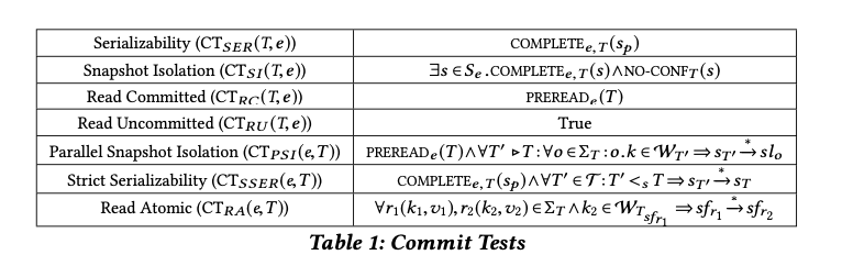
The commit tests for each isolation level are summarised in the table below:
Understanding the snapshot isolation family
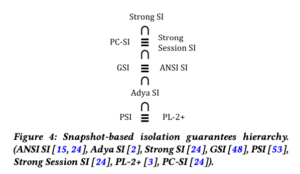
In section 5.2 Crooks et al. use the state-based lens to examine the family of snapshot based guarantees that have grown up over time, including ANSI SI, Adya SI, Weak SI, Strong SI, Generalized SI, Parallel SI, Strong Session SI, Lazy Consistency (PL-2+) SI, and Prefix-Consistent SI. They find that these definitions can be compared on three dimensions:
- time: are timestamps logical or based on real-time?
- snapshot recency: is the snapshot required to contain all transactions that committed before the transaction start time?
- state-completeness: does the snapshot have to be a complete state, or is a causally consistent state sufficient?
Grouping isolation levels in this way highlights a clean hierarchy between these definitions, and suggests that many of the newly proposed isolation levels are in fact equivalent to prior guarantees.
Revealing performance enhancement opportunities
By removing artificial implementation constraints, definitions in terms of client-observable states gives implementers maximum freedom to find efficient strategies. The classic definition of parallel snapshot isolation (PSI) requires each datacenter to enforce snapshot isolation. This is turn makes PSI vulnerable to slowdown cascades in which a slow or failed node can impact operations that don’t access that node itself (because a total commit order is required across all transactions). The state-based definition shows us that a total order is not required, we only care about the ordering of transactions that the application itself can perceive as ordered with respect to each other. In simulation, the authors found a two orders of magnitude reduction in transaction inter-dependencies using this client-centric perspective.
The last word
[The state-based approach] (i) maps more naturally to what applications can observe and illuminates the anomalies allowed by distinct isolation/consistency levels; (ii) makes it easy to compare isolation guarantees, leading us to prove that distinct, decade-old guarantees are in fact equivalent; and (iii) facilitates reasoning end-to-end about isolation guarantees, enabling new opportunities for performance optimization.